Introduction
PSIM is widely used for generating e-drive efficiency maps due to its speed and reliability in such applications. So far, we have discussed automating such simulations with HyperStudy:
Fast-Track eDrive Efficiency Maps in PSIM | Webinar June 2025
While tools like HyperStudy offer code-free automation, Python remains a powerful and flexible alternative for users without access to such platforms.
With this in mind, this article replicates the workflow of the webinar—this time using Python. The process is divided into three steps, each supported by a dedicated Python script:
- Generate valid torque-speed points within the motor's envelope
- Automate PSIM to solve these op. points to steady state and compute efficiency
- Generate an efficiency map contour from the results of Step2
Step 1: Generating valid torque-speed points for the Efficiency Map
There is a dedicated post on how to easily generate valid torque-speed operating points inside the motor envelope:
Generating Valid Torque-Speed Points for PSIM Efficiency Maps with Python
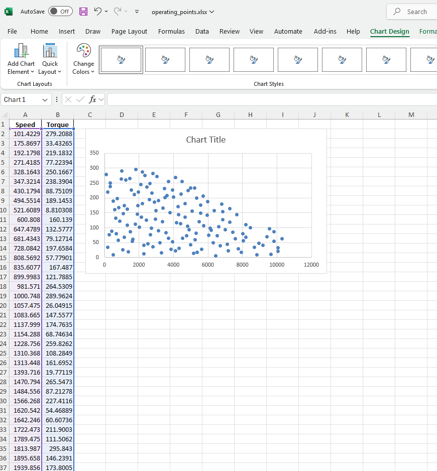
The output of this workflow will be an Excel file containing torque-speed pairs. The 1st column contains the "Speed" and the 2nd column the "Torque" points.
Step 2: Automating PSIM Simulations for Envelope Operating Point Coverage
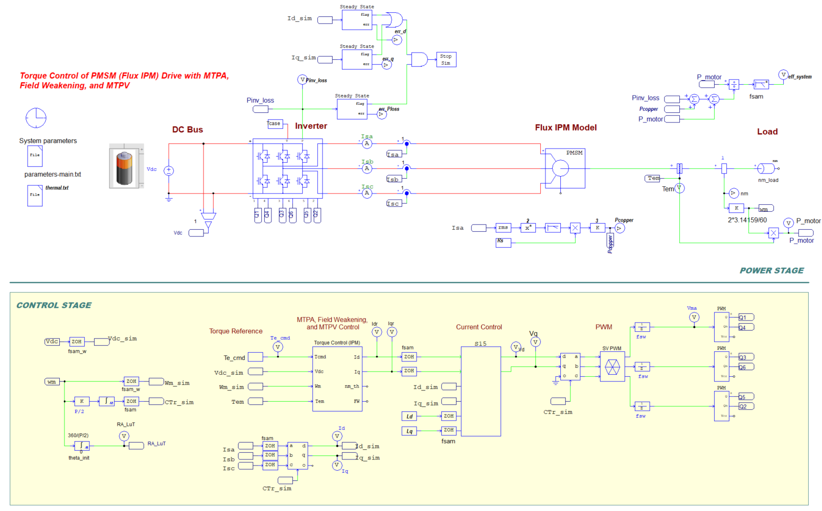
The Excel file from the previous step serves as the input for the second step. Before moving on to the PSIM calls via Python, let's first discuss the e-drive that we will simulate and automate across multiple op. points.
The system is the Linear PMSM drive featured in this webinar:
Fast-Track eDrive Efficiency Maps in PSIM | Webinar June 2025
Note: Please watch the webinar for deeper insights into the system and recommendations for achieving steady state at all operating points. This article just covers the Python automation part.
PSIM simulation file:
Python script to automate PSIM simulations:
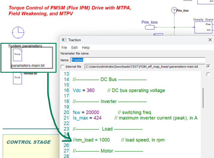
Note: Before running the script, make sure to open the parameter file inside the schematic and comment out the speed (nm_load) and torque (Te_cmd) parameters so they can be parsed from inside the Python script.


I will now briefly explain how the script works:
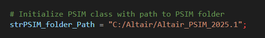
- After opening the script in VSCode, specify the PSIM installation path at line9:
Then click run:
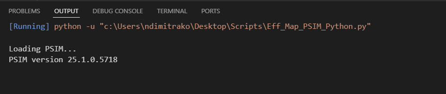
Python will call PSIM to perform a license check, which may take a few seconds but occurs only once. If the license is valid, a PSIM version message will appear. Followed by this tkinter GUI window:
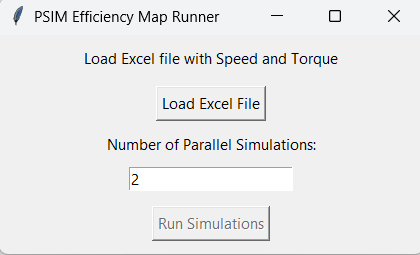
- Then click "Load Excel File" and open the Excel file generated in Step1
- Then define the "Number of Parallel Simulations" - yes, PSIM can run in parallel with the Python PsimASimulate() function at line127
Note: There is an issue with the multi-thread functionality of this function (only for Python) for PSIM v2025.1 and earlier which will be fixed starting from v2026—so pease update to the latest version!
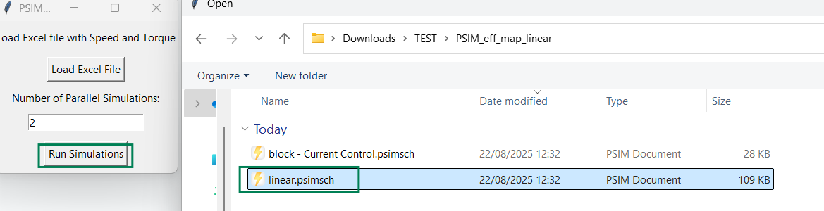
- Click "Run Simulations" and select the motor drive "parent" schematic:
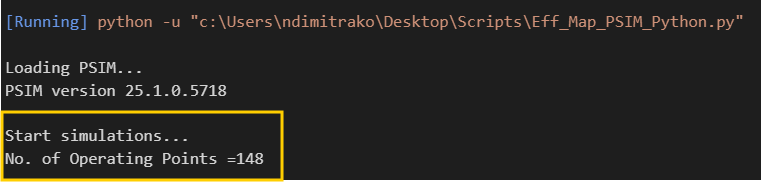
- The following message will appear in VSCode once the simulations start:
- A folder named 'graphs' will be created in the same directory as your schematic, and the PSIM results for each run will be saved there. Once all simulations are completed, you will receive a completion message, and a new Excel file compiling the Speed-Torque-Efficiency results will be generated in the 'graphs' folder:
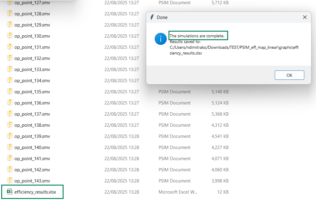
- The generated Excel file will act as input for Step3
Step 3: Generating the Efficiency Map Contour
The final step involves post-processing the Excel file containing the Speed-Torque-Efficiency results into a contour map.
Another custom Python script is provided to streamline this process, using a GUI-based approach built with Python's tkinter library:
After opening and running the script, you will be greeted with this window:
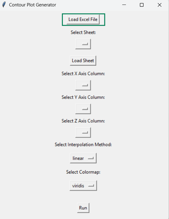
- Click "Load Excel File", navigate to the generated Excel of Step2, and then click "Load Sheet".
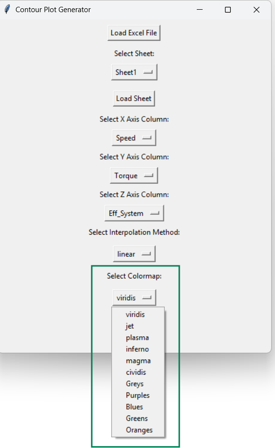
- The Speed will be automatically recognized as the X-axis column, Torque as the Y-axis column and System Efficiency as the Z-axis column (colormap).
- You have two options for the interpolation method of the in-between points (linear or cubic), as well as a list of colormap options to choose from. After selecting your preferences, click 'Run'.
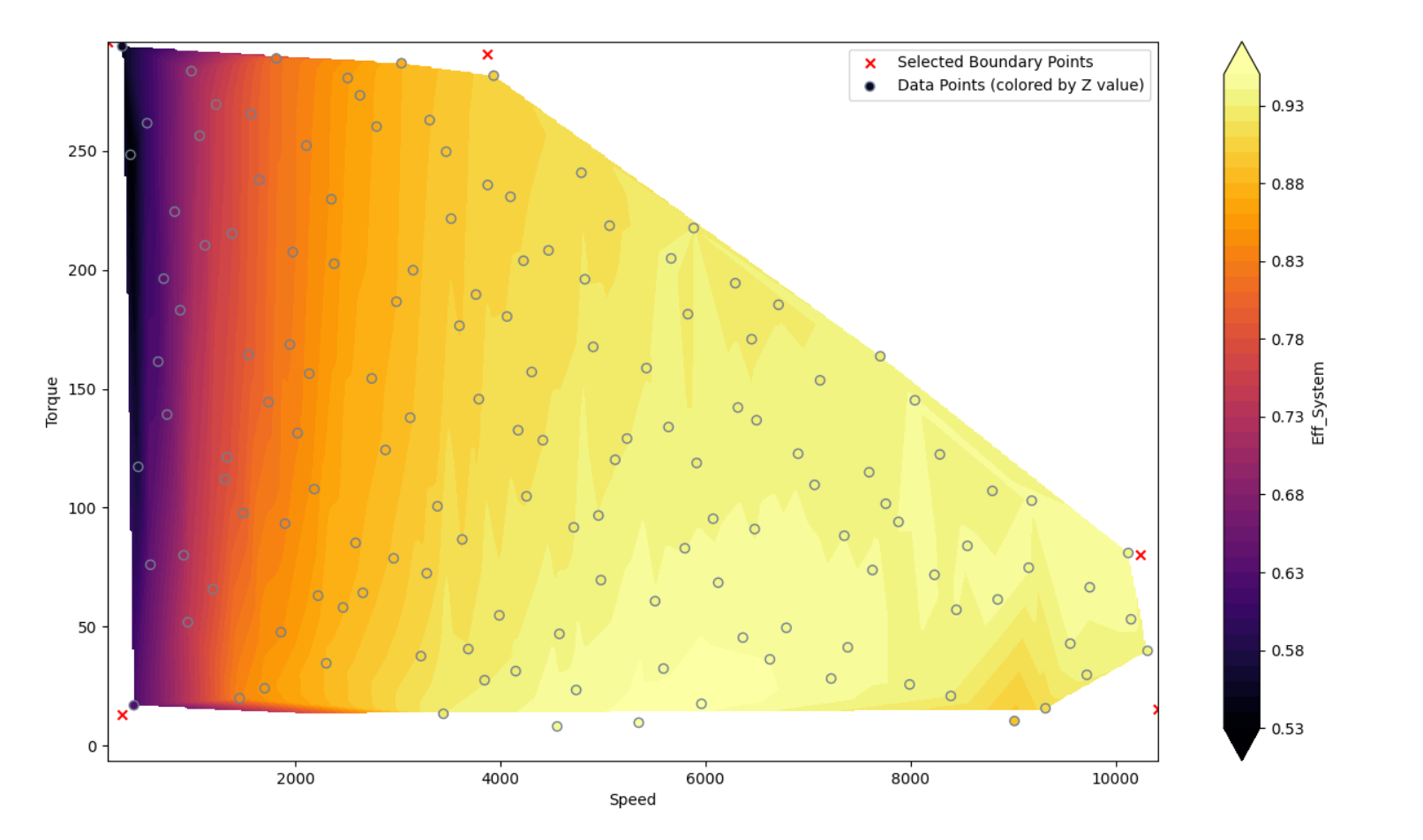
- Then, in the new window that appears, click inside the graph to define the boundary for interpolation. Your clicks will be marked with red crosses:
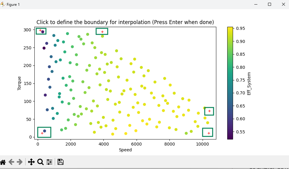
- Once you're done defining the boundary, click "Enter".
- Then, the efficiency map contour will appear:
Note: While Python is user-friendly and widely used, it remains a scripting-based process. This makes debugging difficult when simulations fail to reach steady state or yield unexpected results. In contrast, HyperStudy streamlines debugging and handles much of the "meaningless labor" involved in large-scale simulation automation. For more details, you can take a look in this article: Automating PSIM with HyperStudy vs Scripting
Relevant Links