IntroductionWe will simulate the WLTP Class 3b drive cycle of 1,800sec in just 25sec of simulation time, which is x72 times faster than real time. Let's see how!
Working with drive cycle simulation can be challenging—especially when attempting to include all the details of an electric powertrain.
The main issue arises from the fact that e-drives involve switching power converters operating at high frequencies (in the kHz range). Accurately capturing switching effects, such as inverter switching losses and e-motor PWM losses, requires very small simulation time steps.
Even with a specialized tool like PSIM, which is designed for power electronics (offering features that allow for faster simulations and larger time steps), simulating a full WLTP cycle (e.g., 1800 seconds) can result in very long simulation times.
The trade-off
This leads to yet another engineering tradeoff. Automotive systems are full of tradeoffs, and their simulation is no exception. In this case, we must reduce fidelity in favor of another metric: the fidelity-to-simulation-time ratio.
The goal is to achieve the best combination of accuracy and speed. If a simulation is too slow, it’s impractical. If it’s too inaccurate, it’s useless. We want to maximize the balance between the two.
PSIM is increasingly being integrated into design space exploration frameworks for this very reason. Motor drive simulations in PSIM can be automated using Python or Compose OML, and can be combined with no-code platforms like HyperStudy:
HyperStudy enables fit models creation (reduced-order models) of e-drives based on PSIM data. This approach allows for rapid trend analysis and system optimization, without relying solely on time-consuming simulations.
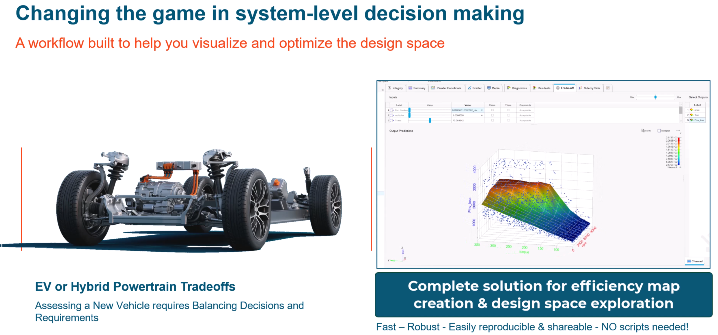
As highlighted in the article “Insights into Motor Drive Design: Analyzing Trends and Long-Term Costs with PSIM and HyperStudy”, focusing on broader system trends and tradeoff exploration often leads to more actionable insights than single (super high fidelity) simulations.
Efficiency Map to Fit Models
The answer to the fidelity vs simulation time trade-off lies in using HyperStudy fit models generated from PSIM system-level efficiency maps.
The process consists of three key steps:
- Efficiency Map Creation from PSIM Simulations
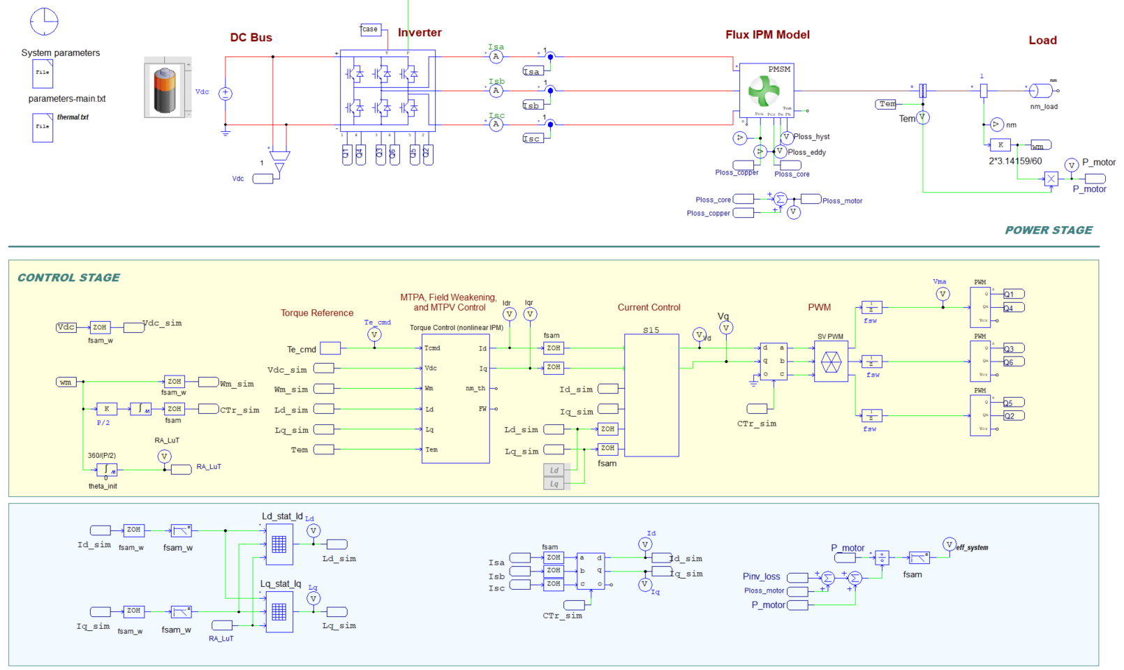
This involves creating a system-level motor drive efficiency map that includes both inverter and motor losses. The map can be "multidimensional", capturing variations across semiconductor devices (e.g., IGBT vs. SiC MOSFET), switching frequencies, modulation techniques, and motor designs. This is what makes the PSIM-HyperStudy combo special!
A dedicated webinar and simulation files on this topic are available here:
Fast Track eDrive Efficiency Maps & WLTP drive cycle with PSIM | Webinar June 2025
Everything that follows is based on this e-drive setup in PSIM. HyperStudy is automating this simulation (found in webinar files):
- Creating the HyperStudy Static Fit Model
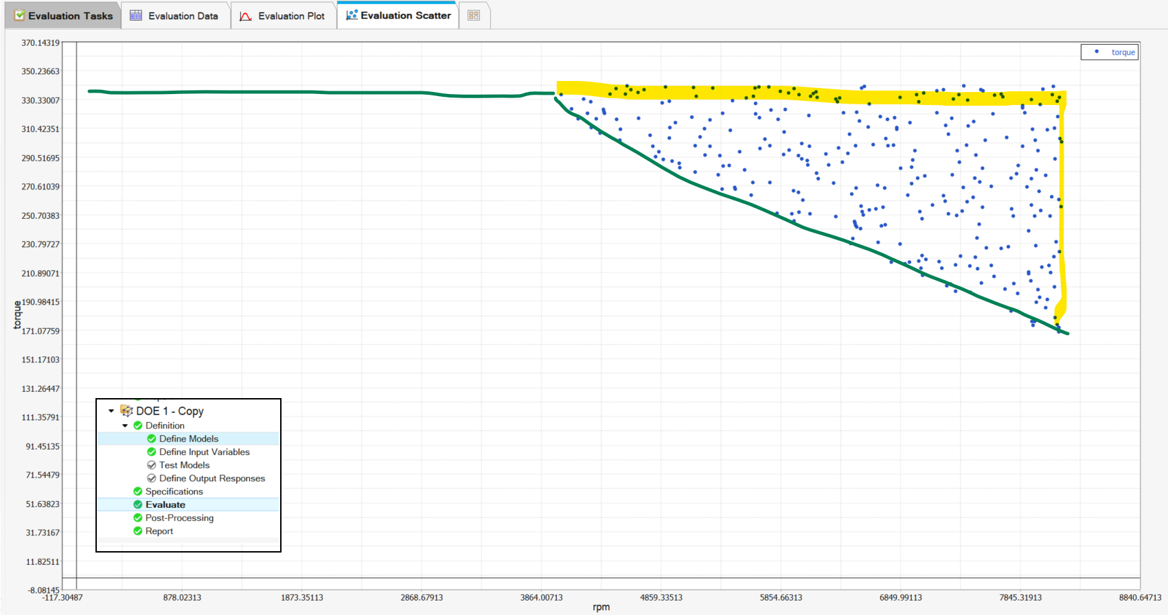
The webinar guides you up to the initial DOE (Design of Experiments) setup of the efficiency map (minute 25 to 35). Creating a fit model from this DOE is quite straightforward.
It involves generating a second, less dense DOE that includes just a few points outside the torque-speed envelope. This is necessary because the fit model algorithm works best with square-distributed data, while the motor envelope, comprising the constant torque and field-weakening regions, is not square.
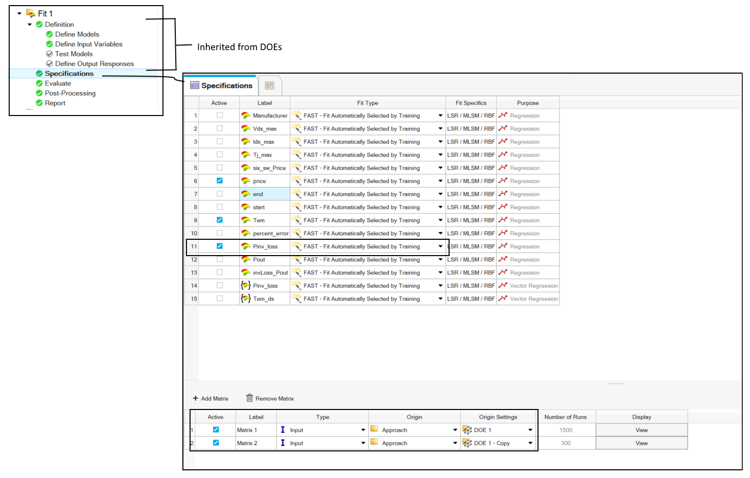
Then we right-click in the "Study Explorer" and click Add » Fit Existing Data » Definition from DOE1 or DOE1-Copy (to inherit the study definition steps up to the "Specifications" section)
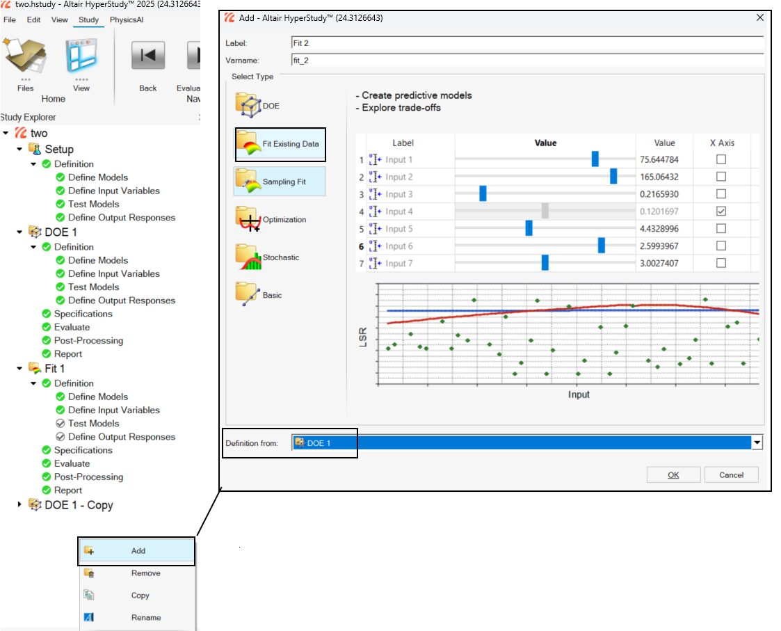
In the "Specifications" section, we select the single output value ("Output Response") for which we want to build the fit model. Let HyperStudy determine the best fitting method by choosing the "FAST – Fit Automatically Selected by Training" option, and then click "Apply" followed by "Next" at the bottom right of the window. Please make sure that the DOE1 and DOE1-Copy data are used in the "Origin Settings" option, as shown below.
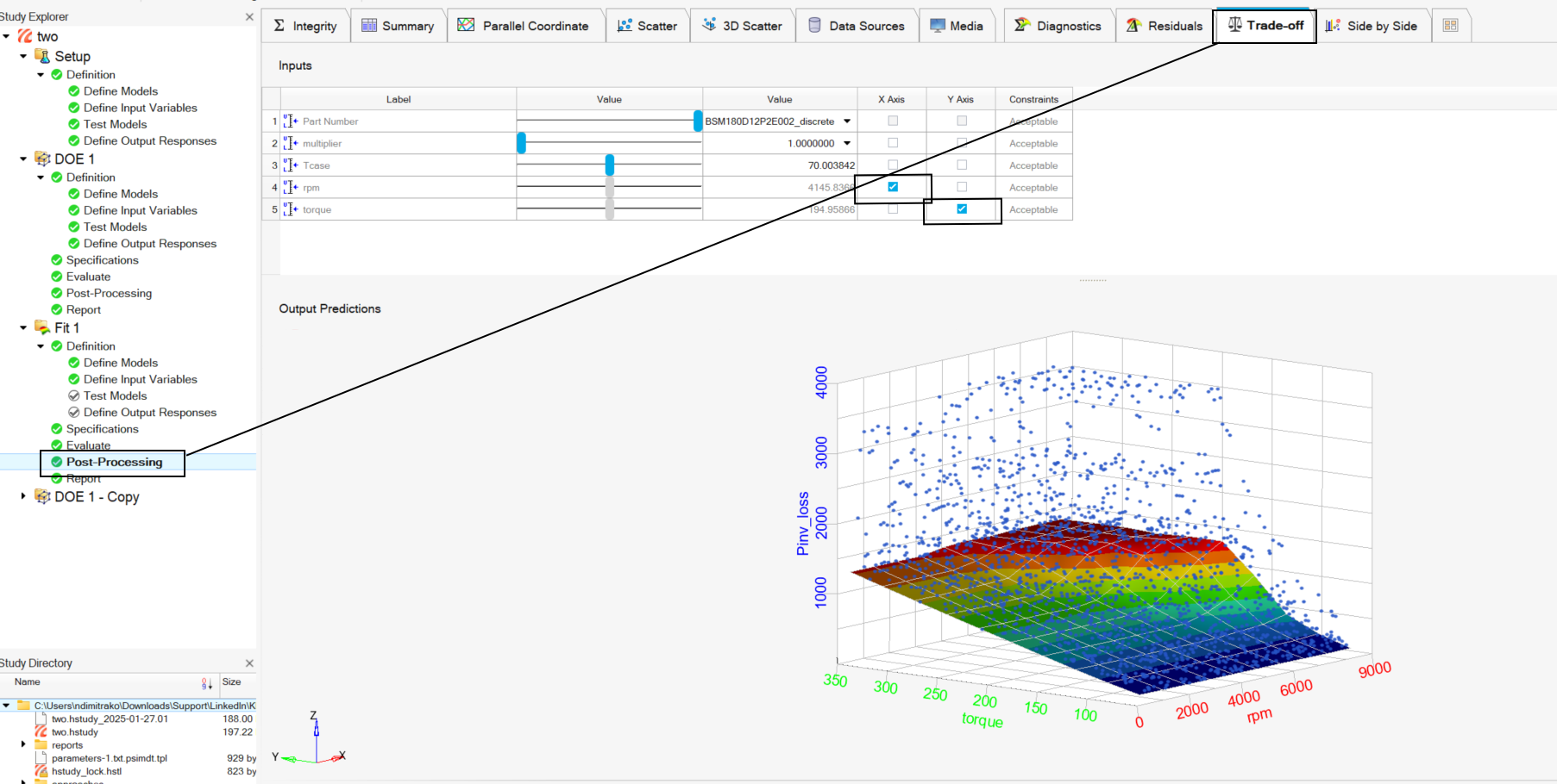
The next step is the "Evaluate" section, where you can just click "Evaluate Tasks" at the bottom right of the window. Once the Evaluation (Fit Model creation) is complete, you can navigate to the "Post-Processing" section. Then navigate to the "Trade-off" tab and mark the speed and torque as the X and Y axis, respectively.
That’s it! You can now explore the design space and system-level trade-offs using dropdown menus and sliders for input variables. For example, in the image below, you can adjust the inverter semiconductor Part Number, Case Temperature (linked to cooling), and Gate Resistance (for EMI vs. switching loss trade-offs).
You can follow this video for the aforementioned steps starting at minute 3:06
Import user DOE data in HyperStudy to perform data-mining and fit creation
This model is a reduced-order representation that approximates the system's losses & efficiency behavior based on key input variables such as torque, speed and other system-level choices.
- Deployment in System-Level Simulation Tools
The final step is exporting this fit model in a meaningful way to be deployed in a system level integrator tool such as Altair Twin Activate or Matlab Simulink.
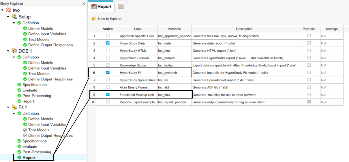
To do that, you can navigate to the "Report" section in HyperStudy and select to export as:
- As a *.pyfit file for Altair Twin Activate
- As a FMU (Functional Mock-up Unit) for Simulink or other FMI-compliant tools
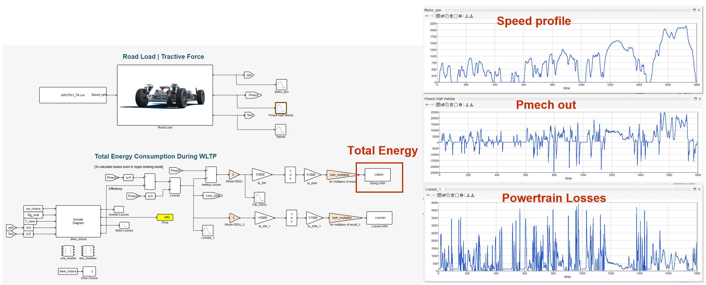
The following example is within Altair's Twin Activate system integration platform. We can deploy the PyFit model using the "HstPyFitBlock". In this case, I am using the "Include Diagram" block to switch between the two drive systems investigated in this article with a single variable:
Kia EV9: A quick look into the Dual Inverter Strategy with PSIM
We can then calculate system-level efficiency and total losses for a WLTP drive cycle using arbitrary vehicle road load coefficients.
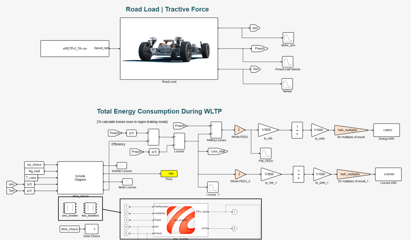
This integration allows complete drive cycle simulations to be performed, including road load models, vehicle dynamics, and speed profiles, without resolving individual switching events. The simulation runs with larger time steps, drastically reducing compute time, while still accurately reflecting motor and inverter losses due to the PSIM trained fit model.
The simulation solves a WLTP drive cycle of 1,800 seconds in just 25 seconds, which is x72 times faster than real time.
This concludes the creation of the Efficiency Map Fit Model using PSIM and HyperStudy, which is the first part of this workflow. The workflow continues in Part 2:
Faster-than-Real-Time EV Drive Cycle Simulations with PSIM-trained Fit Models | Part2
Relevant links:
- Fast Track eDrive Efficiency Maps & WLTP drive cycle with PSIM | Webinar June 2025
- Fit Model use for design decision-making | Altair Power Conversion Webinar Feb 2025
- Insights into Motor Drive Design: Analyzing Trends and Long-Term Costs with PSIM and HyperStudy
- Kia EV9: A quick look into the Dual Inverter Strategy with PSIM
- Accelerate your power converter design with PSIM & HyperStudy | Tutorial
- Automating PSIM with HyperStudy vs Scripting
- Flux-PSIM Coupling : Leverage the system simulation speed while working around your Motor Design
- Optimizing Washing Machine Control with Power Electronics and Multi-Body Dynamics Integration