Type 3 Controller Optimization - Part 1

In this article we will explain how to set up the optimization of a Type 3 Controller with PSIM and HyperStudy.

Note: Part 2 has been uploaded and adds Phase Margin and Crossover Frequency to the optimization.

The first thing we need to do is to define our variables (inputs) and goals for the optimization so that we can set them in HyperStudy later:

Optimization Inputs

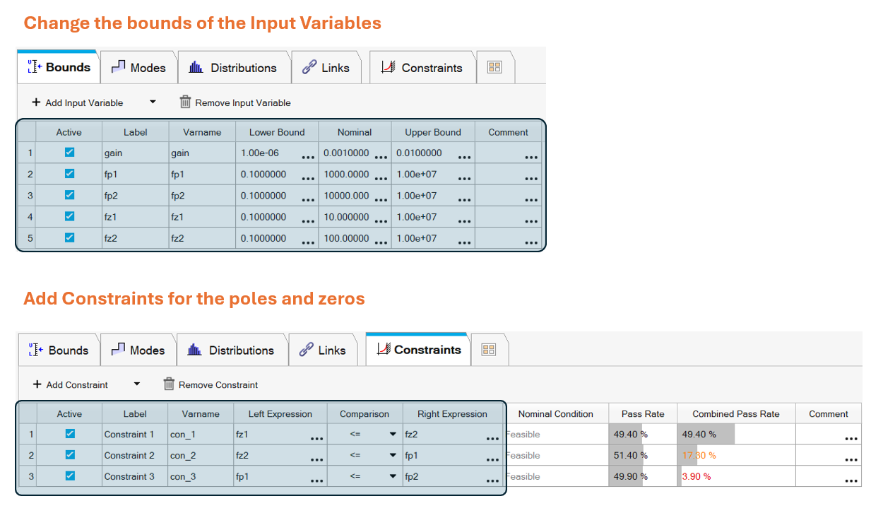
The optimization inputs are the variables which are going to be explored to achieve the goals we set, ranges and relationship between these also must be defined.

Additional to the bounds, we also need to specify other qualities for these input variables. For this application, the frequency of the zeros needs to be less than those of the poles:

fz1 > fz2 > fp1 > fp2

Optimization Goals and Constraints

For this example, a set of qualities from the output waveform were chosen as KPIs (Key Performance Indicators) to improve. In HyperStudy, goals are either to minimize or maximize a variable. So, constraints on these goals must be set to get useful values at the end.

Additional Constraints

Since the change in the inputs can have undesirable outcomes in the output waveform a set of additional constraints were implemented:

Steady State Detection: The circuit includes a block that detects steady state and raises a flag, therefore we set up HyperStudy to check it.

Modulation Waveform Ripple: Harmonic and subharmonic oscillations in the modulation waveform can cause multiple issues in the circuit, therefore an amplitude restriction was set to prevent this.

Now, let us look at how implementation looks like with PSIM and HyperStudy

PSIM Schematic

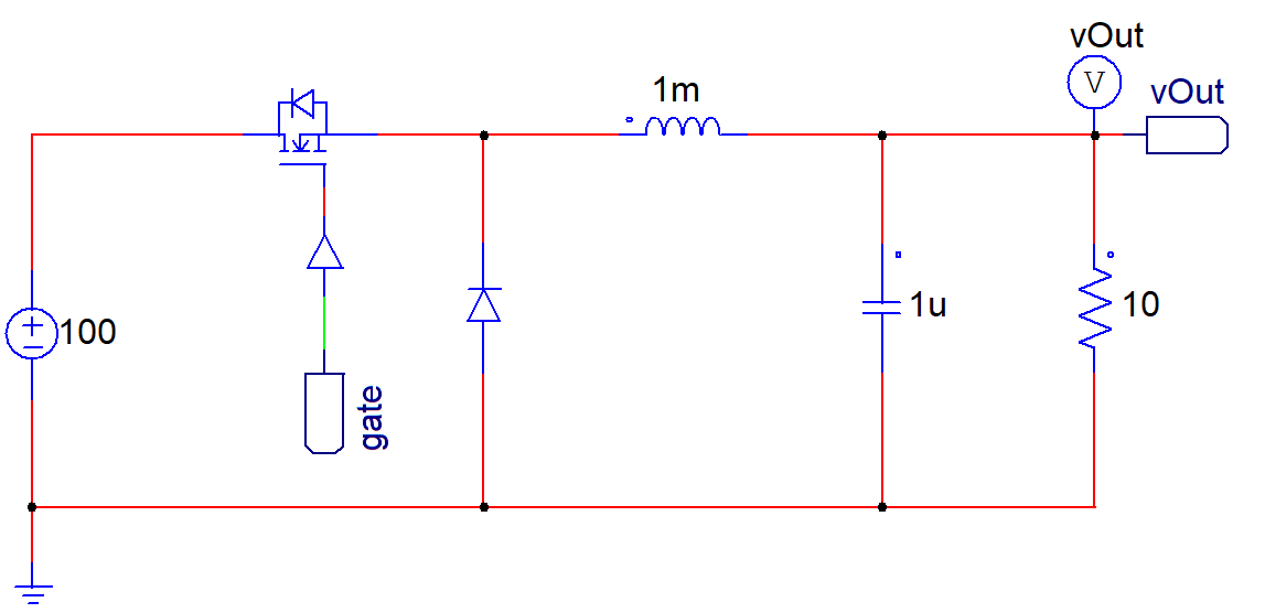
The PSIM schematic is composed of three main parts:

• Buck converter with Ideal switching devices:

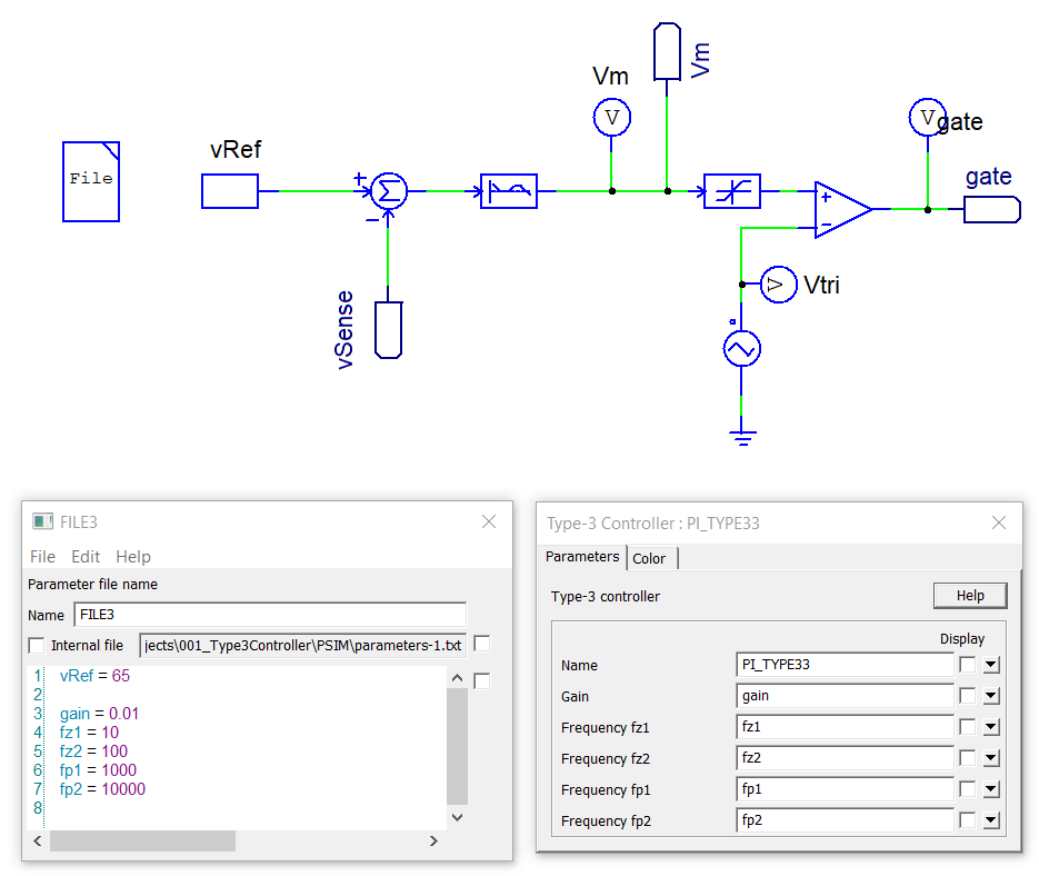
• Type 3 Controller with PWM generator:

The Type 3 Controller Block has been parametrized for the gain, poles and zeros using a parameter file.

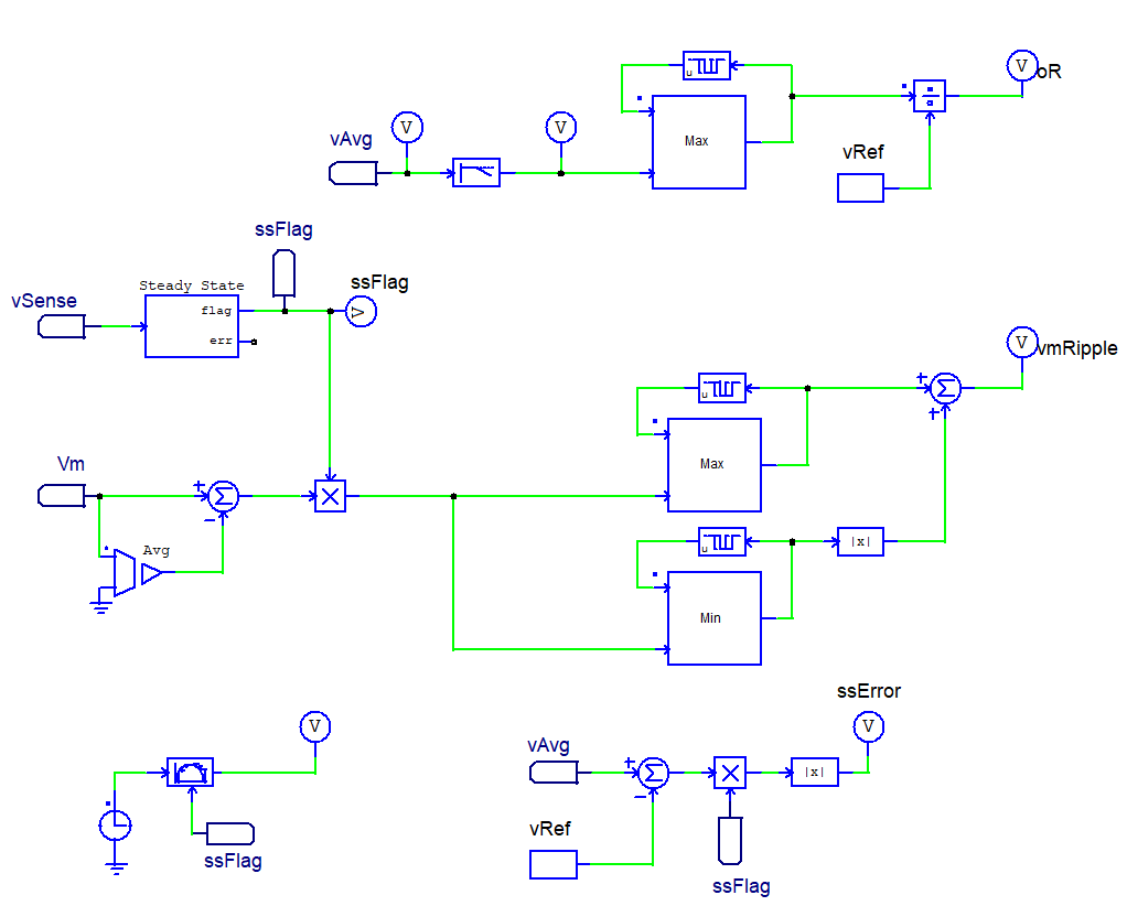
• Measurement blocks and circuits

These blocks measure everything we mentioned in the Goals and Constraints sections.

HyperStudy Optimization Setup

The first step is to add a PSIM model to a new study and import the input variables.

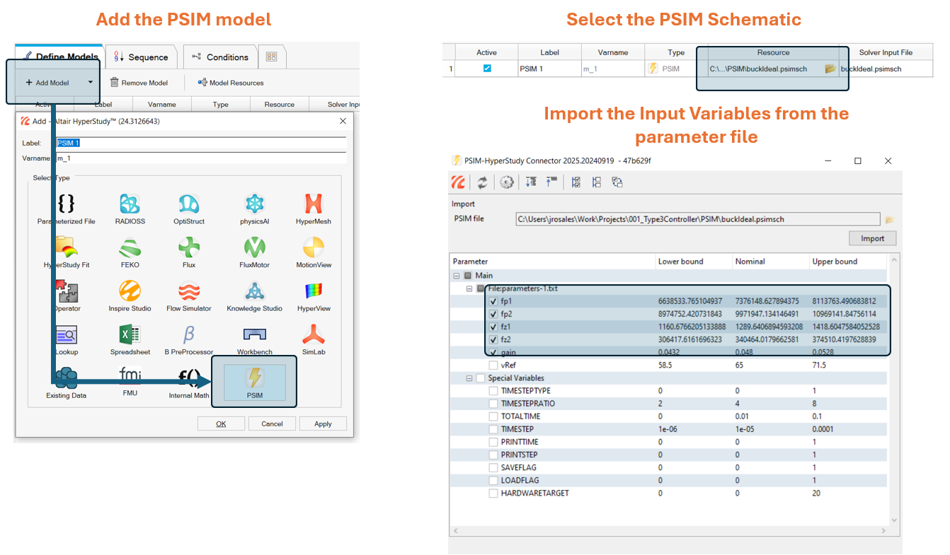
Then, we need to define the bounds for the input variables and the constraints, these are the ones proposed in the first section of this article:

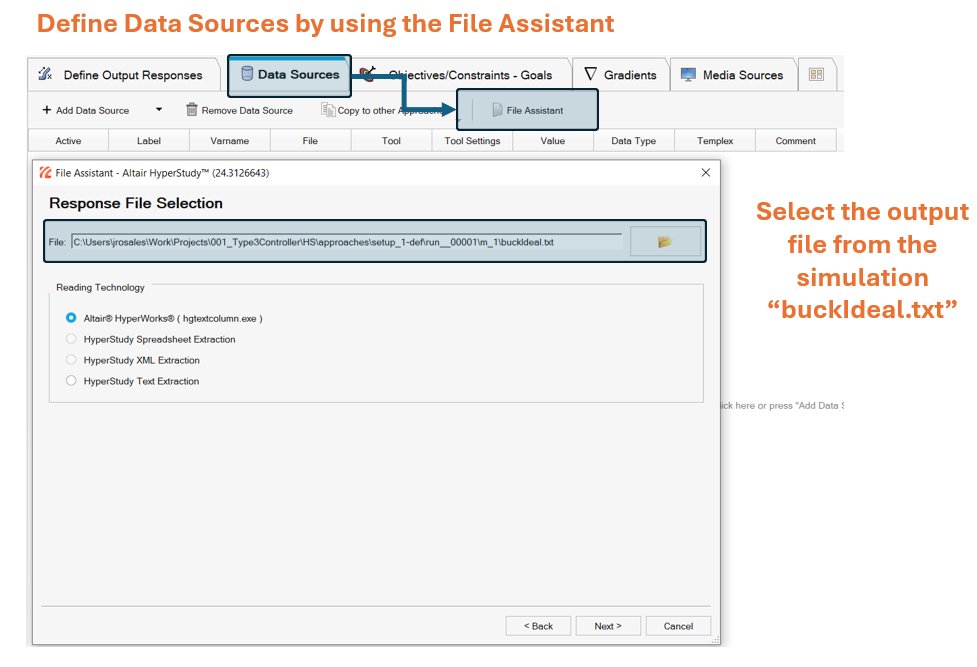
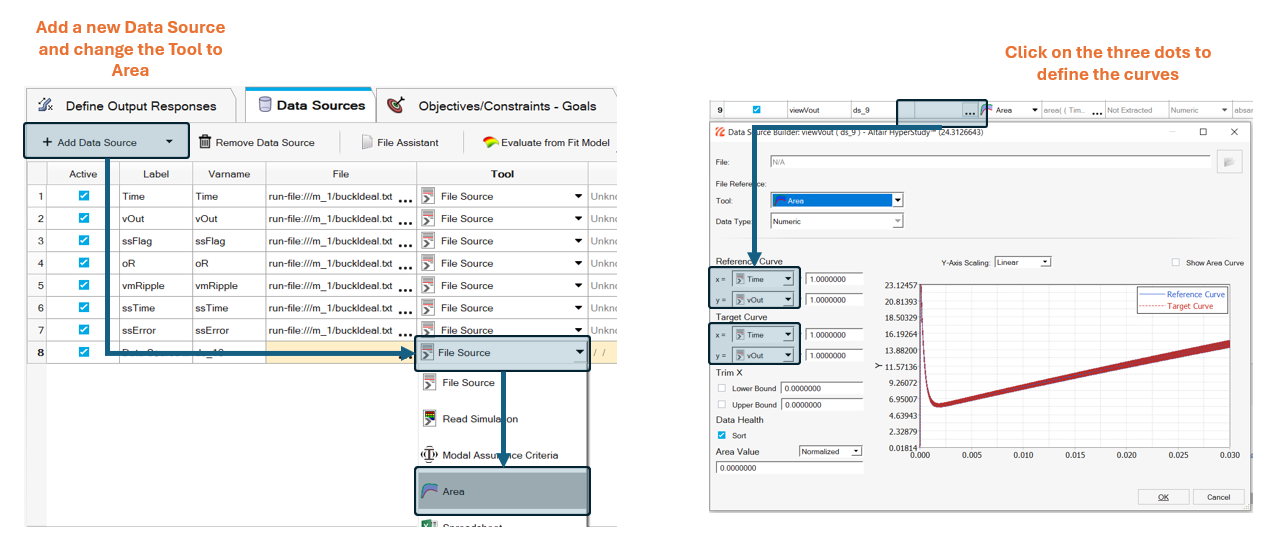
After executing the Test Model, perform the extraction of Data sources from the output file:

Add the following curves to the data sources:

• Time
• vOut – Output Voltage
• ssFlag – Steady State Flag
• oR – Overshoot Ratio (use (max(oR)-1)*100 to get the percentage)
• vmRipple – Peak to Peak amplitude of modulation waveform
• ssTime – Settling Time measurement
• ssError – Steady State Error

Use the data sources to define the Output Responses, the default operation (“max(var)”) is good enough for how these characteristics are measured in PSIM:

Note: adding a data source automatically creates an output response

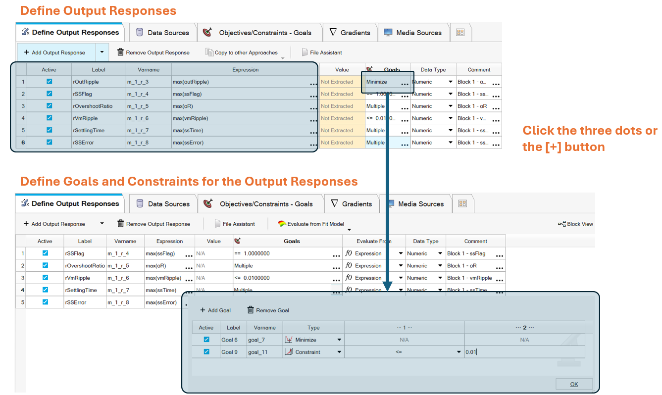
With the Output Responses defined we can finish the setup.

The last step is creating an optimization with the setup as a source (Right Click on Study Explorer > "Add").

From the "Specifications" tab, we just need to select GRSM as the optimization method and use the default number of evaluations.

Finally, from the "Evaluate" tab, start the process.

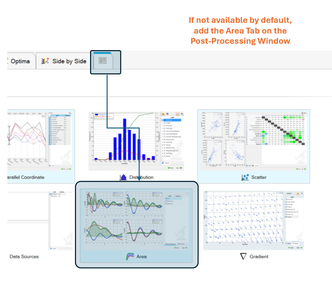
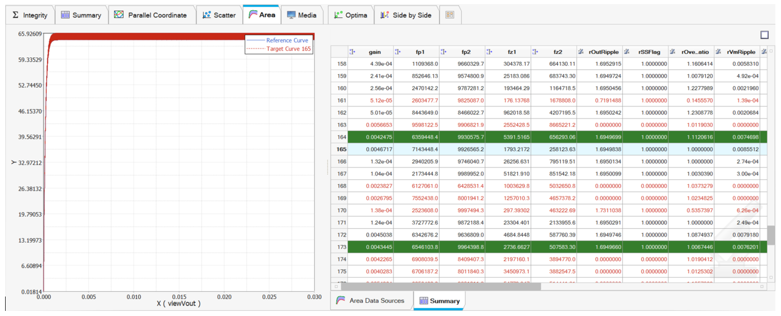
After all evaluations are completed (in the "Post-Processing" window), use the Area tab to sweep through all iterations. Rows in Green are the most optimal values.

You can find the PSIM schematic and the HyperStudy setup here:

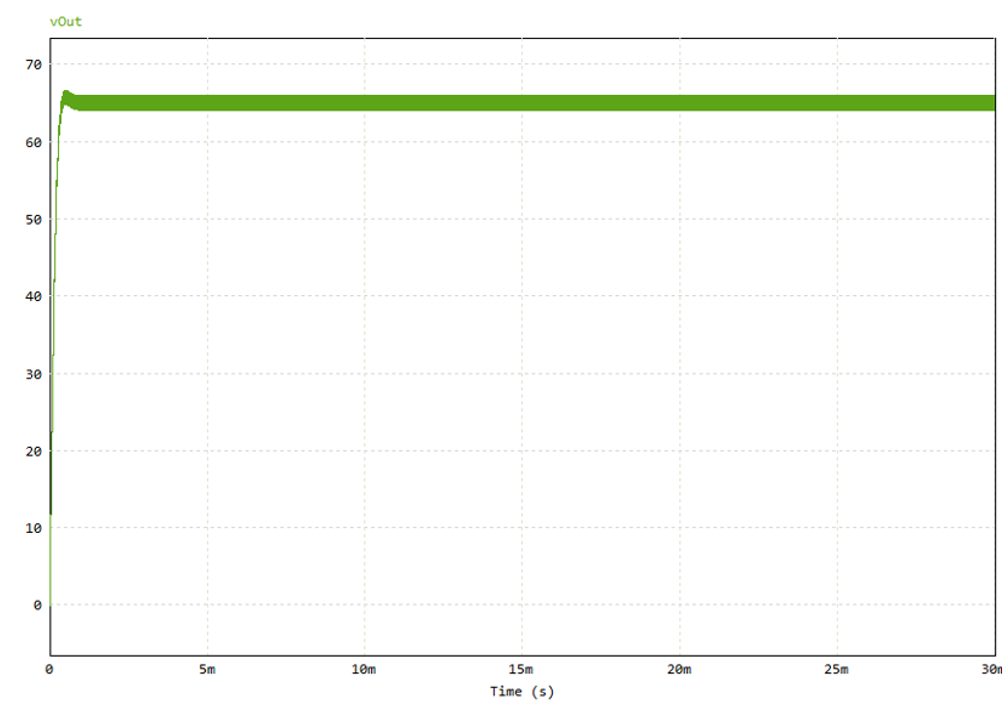
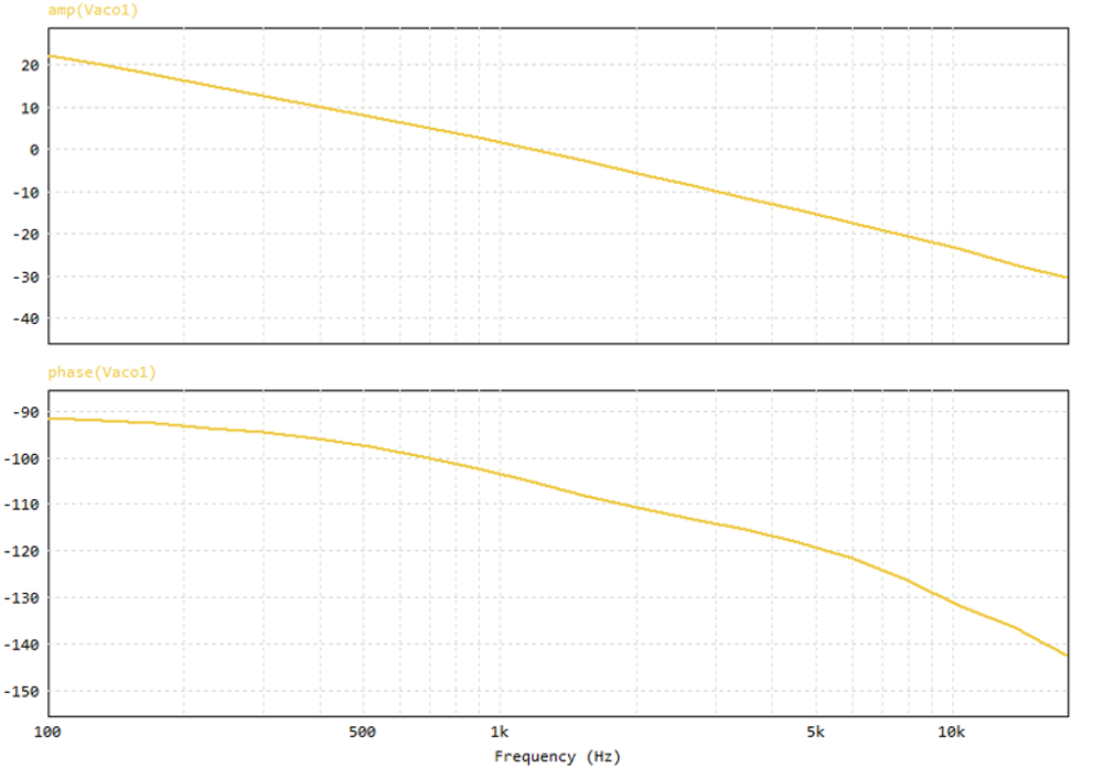
Here's one of the optimized results and it's closed loop response:

Area Tool to view output voltage plots

If we create a Data Source with the Area Tool, we’re going to be able to see each all output voltage waveforms from each iteration of the optimization, we just need to add the Time and vOut vectors to both the reference and the target curve.

Note: This is not the intended use for the Area tool but provides easy access to the output waveforms of the converter