Overview:
Accurately simulating real-world scenarios involving moving objects is a complex yet crucial task. One such challenge is modeling the aerodynamic behavior of a train moving through a tunnel, where pressure waves, turbulence, and transient airflow interactions play a significant role in design and safety considerations.
AcuSolve, which is Altair’s general-purpose CFD solver, leverages advanced moving mesh technology to tackle such dynamic simulations with precision and efficiency. This innovative approach moves the existing mesh nodes, as opposed to the traditional remeshing approach, which makes the solver faster, and introduces fewer errors in the process. This allows engineers to capture the intricate flow characteristics around moving bodies without remeshing and the associated interpolation errors.
In this example, we can see how AcuSolve’s moving mesh capabilities enable the realistic simulation of a high-speed train traveling through a tunnel.
Prerequisite:
This article assumes the knowledge of concepts shown in the following tutorial:
https://help.altair.com/hwcfdsolvers/acusolve/topics/tutorials/acu/acu_5202_intro_sl_r.htm
The steps shown in this article assumes that mesh exists by using appropriate mesh controls. You can find the mesh controls in the attached .slb file.
Usage/Installation Instructions:
Step 1
Create a ‘Transient’ flow solution

Note that a moving mesh is needed for this model, and the Moving body is ‘Specified’, which means that the user needs to specify the motion of the nodes, during the mesh motion (done in Step 8).
A multiplier function of the type “piecewise linear” is used for timestep size.

This timestep multiplier is employed, to accelerate the solver when the train is outside the tunnel, and solution is more accurate in the time period when the train is inside the tunnel.
Step 2
Assign materials to both the ‘moving region’ and the ‘fixed region’


As the train is moving at a relatively high speed, using the constant property model for ‘Air’ would not be ideal. The isentropic material model, takes into account compressibility effects.
Step 3
Apply inlet boundary conditions to the inlet face

Since there is no forced air flow from the inlet face, using a 0 Stagnation Pressure boundary condition is the most appropriate. ‘External’ turbulence flow type is used since the face is an external environmental pseudo-face in which the expected eddy viscosity is very low. If you would expect a larger eddy viscosity value, use ‘Internal’ turbulence flow type.
Step 4
Create ‘Outlet’ boundary condition

Use a 0 pressure boundary condition at the outlet face.
Step 5
Create ‘Slip’ faces

Use ‘slip’ boundary condition on all the faces of the geometry that represents the environment and are not physical faces.
Step 6
Use ‘Wall’ boundary conditions for the train and the tunnel


Step 7
Apply ‘Mesh Motion’ on the train

Note that the train speed has the following multiplier function (note the aim of the current article is to demonstrate mesh motion and other solver capabilities, while keeping the runtime low, hence the acceleration profile)

This multiplier function enables the train to move with a constant acceleration from 0 to 1 second, then constant velocity from 1 to 4 seconds, and finally constant deceleration until it comes to stop from 4 to 5 seconds.
Step 8
Apply Nodal Boundary conditions
Go to Advanced BC -> Nodal Boundary conditions.

Since the solution definition has ‘Specified’ mesh motion in Step 1 of this article, we specify the mesh motion in this boundary condition. Here, the mesh displacement is desired in the Y direction, so the variable is ‘Mesh Y displacement’. The goal is to not distort the mesh elements close to the train geometry, however, the elements in front of the train must be squeezed, and the elements behind the train must be stretched. At the same time, the elements on/near the train must translate but not change in size. This can be achieved by a ‘Piecewise Linear’ type for the boundary condition. A curve needs to be defined for the nodal movement multiplier, like the following:
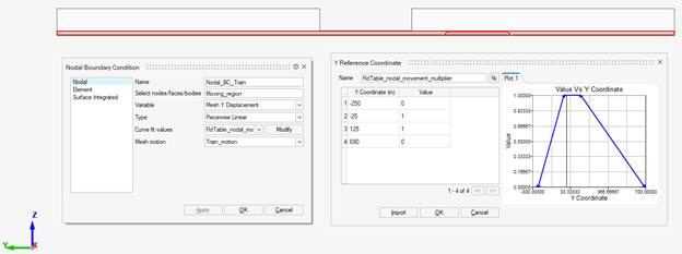
The train is 100m long and the train is positioned between Y-coordinates 0 to 100. To account for some elements ahead and behind of the train to move with the train, and to not distort them, the above multiplier is chosen where 25m ahead and behind the train will have similar motion as the train itself (hence the values -25 and +125).
The Y-coordinates at the end of the simulation domain (-250 and +650) are given a value of 0, which means that the elements on those coordinates will be fixed. The Y-coordinates between -25 and +125 are given a value of 1, which means that the elements in those coordinates will move 1:1 along with the mesh motion specified (without any element distortion). Finally, all other elements in between -250 and -25, and all elements between +125 and +650 will have an intermediate (linear) value describing the motion of those elements.
Step 9
Run the model
Right-click on ‘Results’ and ‘Update Solution’.
Post-Requisite:
The results can be visualized within SimLab.
Velocity contours can be plotted like below.

The mesh deformation can also be visualized like below: