OS-T: 1600 Fluid-Structure Interaction Analysis of Piezoelectric Harvester Assembly
Product Version: Hyperworks 2021.2.1 or above
The purpose of this tutorial is to demonstrate how to carry out Fluid-Structure Interaction analysis that is, with OptiStruct nonlinear transient analysis coupling within AcuSolve fluid dynamic analysis.
In this tutorial, you will explore the possibility of using piezoelectric based fluid flow energy harvesters. These harvesters are self-excited and self-sustained in the sense that they can be used in steady uniform flows. The configuration consists of a piezoelectric cantilever beam with a cylindrical tip body (which is the structure model) which promotes sustainable, aero-elastic structural vibrations induced by vortex shedding and galloping. The structural and aerodynamic properties of the harvester alter the vibration amplitude and frequency of the piezoelectric beam and the fluid flow. As you may know, the Piezoelectric energy harvesting using fluid flow involves the mutual interaction of three distinct dynamic systems, namely the fluid, the structure and the associated electrical circuit.
Note: This tutorial is limited to study only fluid and the structure domain.
Figure 2 illustrates the fluid structural model used for this tutorial: the dimensions of the beam are shown in Figure 1 and Figure 2.
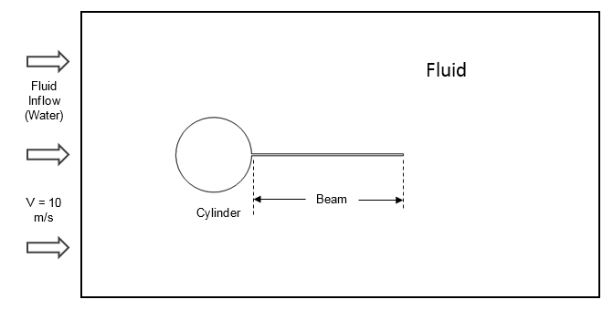
Figure 1. Schematic of the Problem
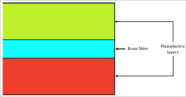
Figure 2. Various Layers of Beam
The AcuSolve fluid model (slab_dcfsi.inp) and the OptiStruct structural beam model (Slab.fem) are located in the fsi_models.zip file. Refer to Access the Model Files in the online help.
Step 1. Launch HyperWorks and Set the OptiStruct User Profile
- Launch HyperWorks.
- Select OptiStruct solver interface.
This loads the user profile. It includes the appropriate template, macro menu, and import reader, paring down the functionality of HyperWorks to what is relevant for generating models for OptiStruct.
Step 2: Import the Model
- Click File > Import > Solver Deck.
A Select OptiStruct file browser opens.
- Select the Slab.fem file you saved to your working directory.
- Click Open.
- Click Import to close the Solver Import Options window.
Step 3: Set Up the Model
3.1 Create Contact Surface
- In the contact Browser, right-click and select Create > Contact Surface from the context menu.
A default contact surface template displays in the Entity Editor.
- For Name, enter FSI_Interaction_Surf.
- Click Color and select a color from the color palette.
- For Elements, click 0 elements > elements > face and pick all the faces of the beam except in the front and end faces, as shown in Figure 3.
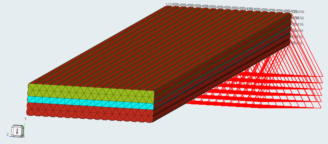
Figure 3. All sides of the beam except in the front
- Click
 to add the faces to the contact surface.
3.2 Define Nonlinear Parameters
- In the Model Browser, right-click Load Step Inputs collector and select Create > NLPARM, as shown in Figure 4.
A default NLPARM load step inputs collector template displays in the Entity Editor.
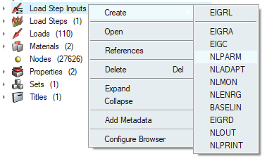
Figure 4. Create NLPARM card
- For Name, enter NLPARM.
- Input the values, as shown in Figure 5.
See NLPARM Bulk Data Entry for more information.
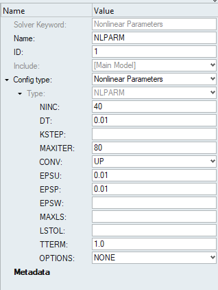
Figure 5. NLPARM card
3.3 Define Transient Time Step Parameters
- In the Model Browser, right-click Load Collectors and select Create > TSTEP.
A default TSTEP load collector template displays in the Entity Editor.
- For Name, enter TSTEP.
- For TSTEP_NUM, enter 1.
- Input the values, as shown in Figure 6.
See TSTEP Bulk Data Entry for more information.
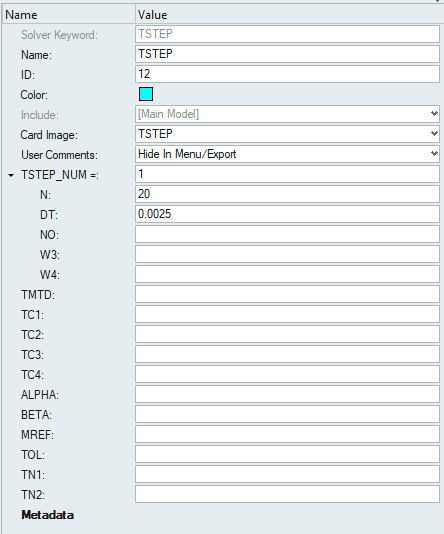
Figure 6. TSTEP card
3.4 Define Incremental Result Output for Nonlinear Analysis
- In the Model Browser, right-click Load Step Inputs collector and select Create > NLOUT.
A default load step inputs collector template displays in the Entity Editor.
- For Name, enter NLOUT.
- Input the values, as shown in Figure 7.
See NLOUT Bulk Data Entry for more information.
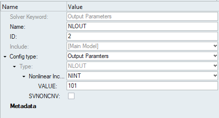
Figure7. NLOUT card
3.5 Define Fluid-Structure Interaction Parameters
- In the Model Browser, right-click Load Collectors and select Create > FSI.
A default FSI load collector template displays in the Entity Editor.
- For Name, enter FSI.
- Input the values, as shown in Figure 8.
See FSI Bulk Data Entry for more information.
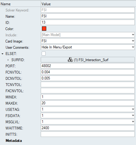
Figure 8. FSI card
3.6 Define Output Control Parameters
- In the Model Browser, right-click cards collector and select Create > GLOBAL_OUTPUT_REQUEST, as shown in Figure 9.
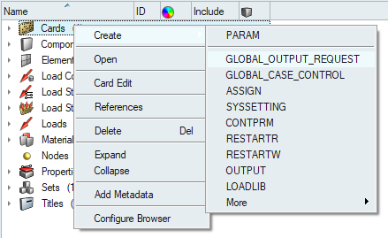
Figure 9. Create GLOBAL_OUTPUT_REQUEST
- For DISPLACEMENT, ELFORCE, OLOAD, STRESS, and STRAIN, set Option to Yes.
3.7 Create Nonlinear Transient Analysis Subcase
- In the Model Browser, right-click and select Create > Load Step from the context menu.
- For Name, enter FSI.
- For Analysis type, select Nonlinear transient.
- Select the Load Collector, as shown in Figure 10.
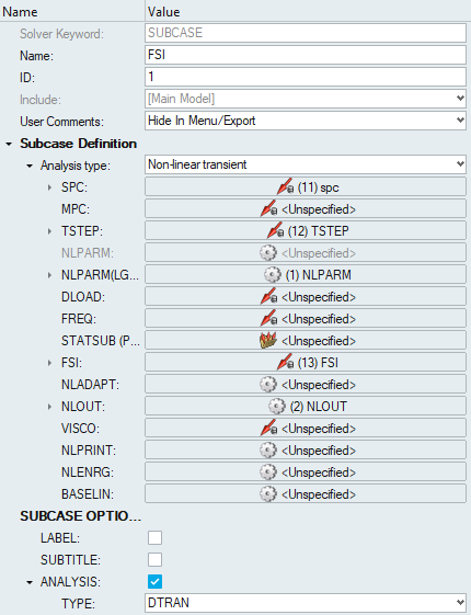
Figure 10. Create load step
Step 4: Modify the AcuSolve input file
- Open the AcuSolve input file (slab_dcfsi.inp) in a text editor.
- Change the socket_host parameter in the EXTERNAL_CODE block to your machines hostname and save the file, as shown in Figure 11.
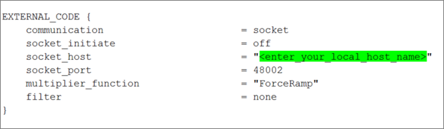
Figure 11. Modify the AcuSolve input deck
Step 5: Submit the Job
- Launch the Compute Console (ACC), select CoSim > FSI AcuSolve, select the Slab.fem file as input file and the slab_dcfsi,inp file as Cosimulation file, as shown in Figure 12.
- Click Run.
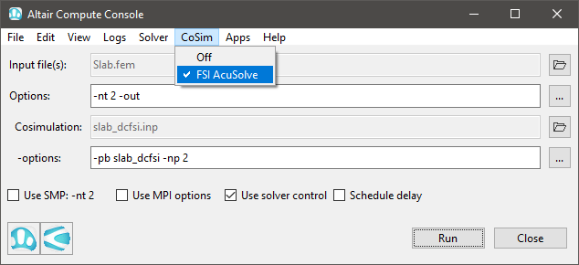
Figure 12. Submit the job using ACC
If the job is successful, you will see new results files in the directory where the input decks are located in. The Slab.out file is where you will find error messages that will help you debug your input deck, if any errors are present.
The default files that will be written to your directory are:
cci.txt
Contains information pertaining to model progression. Logs regarding connection establishment, initial external code handshake and subsequent time step data in conjunction with exchange/stagger.
Slab.html
HTML report of the analysis, giving a summary of the problem formulation and the analysis results.
Slab.out
ASCII based output file of the model check run before the simulation begins and gives some basic information on the results of the run.
Slab.stat
Summary of analysis process, providing CPU information for each step during the process.
Slab.h3d
HyperView compressed binary results file.
Step 6: View the Results
Using HyperView, plot the Displacement contour at 0.95 s, as shown in Figure 13.
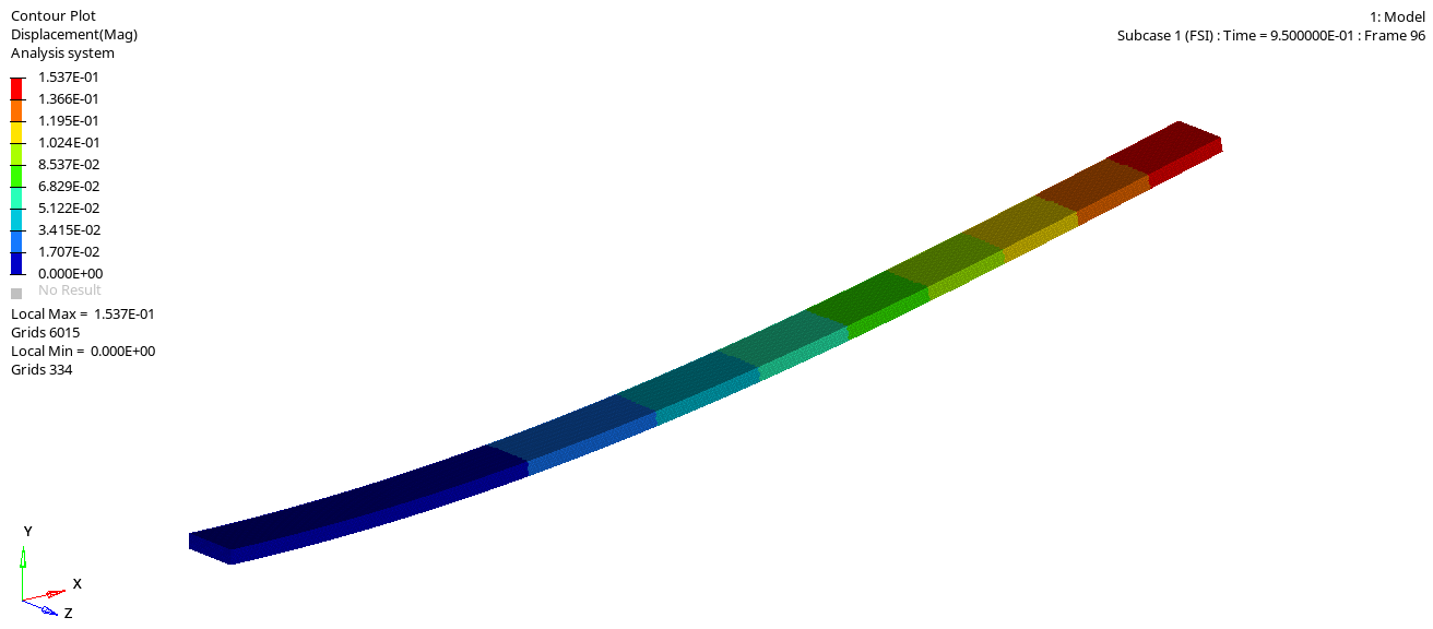
Figure 13. View the Results
