Introduction
Permanent magnets play a crucial role in modern electromechanical devices, ensuring efficient performance in applications ranging from electric machines to sensors. PM motors are now the most used motors in the automotive industry. Optimization is key to improving performance. Recent advancements in simulation tools, such as those provided by Altair Flux, have improved the ability to analyze and optimize easily the use of magnets, allowing engineers to develop more robust designs. We propose to show how to improve performance and minimize the mass of magnets.
Goal of the analysis
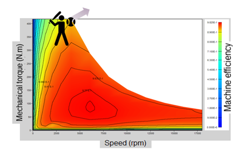
When analyzing PM motors, we often compute efficiency map (see Figure below). We propose here to focus on the base point and check how we can improve it: maximize mechanical power available and minimizing mass of magnets. The mass of magnets is also dealing with cost of motor as the magnet is usually quite expansive compared to other elements of the motor. Decreasing mass of magnets also allows going toward a more sustainable world, decreasing the footprint of human activities.
Key parameters for optimizing base point
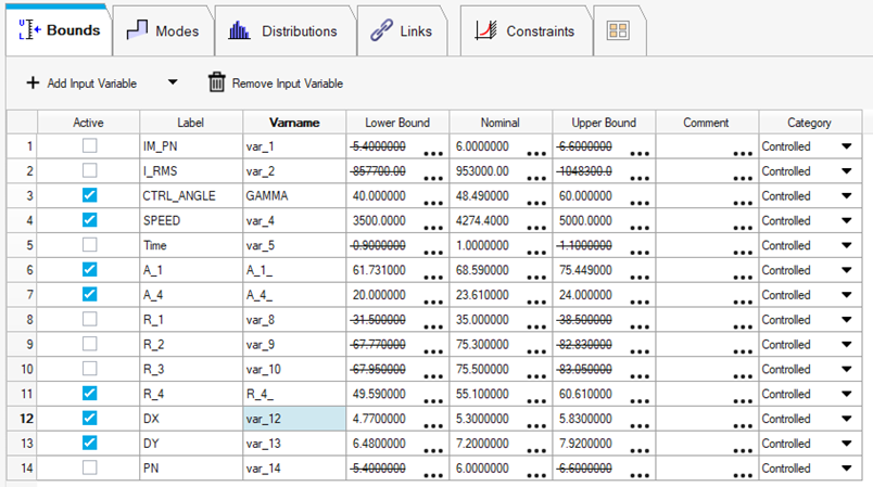
We propose to fix max current and use the speed and the control angle as physical parameters. As regards magnets, a set of parameters will allow modification of magnet shape in the rotor part (see screen shot below).
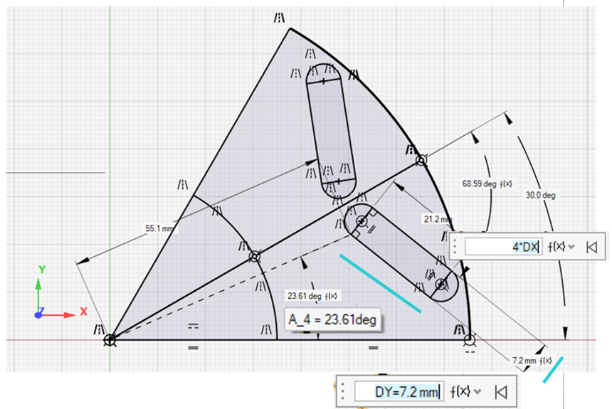
We have dedicated parameters to define shape of the magnet:
- DX : width of the magnet (DX=5.3mm and 4*DX=21.2mm)
- DY : length of the magnet (DY=7.2mm)
- R_4 : radius of one corner of the magnet (R_4=55.1mm)
- A_4 : angle of one corner of the magnet (A_4=23.61 degree)
- A_1 : angle of the magnet (A_1=68.59 degree)
Defining the magnetic project
Then the geometry is ready, all materials and circuits are defined and associated with the required bodies. Parameters can easily be created to be driven by the optimizer to define current angle and speed for instance.

Parameters can easily be created to be driven by the optimizer to define current angle and speed for instance.
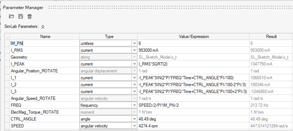
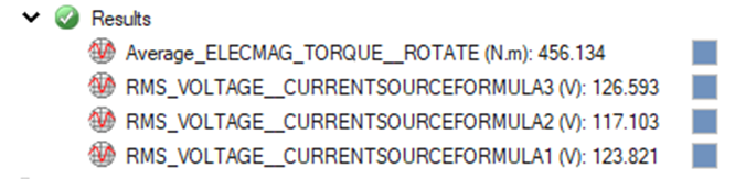
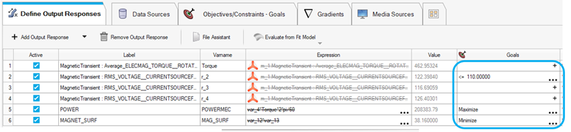
It is also possible to define results which will be used by the optimizer as results.
Optimizing method
Once the project has been defined with all geometric and physical parameters, there is a one click button to open Altair HyperStudy the Altair optimizing tool.
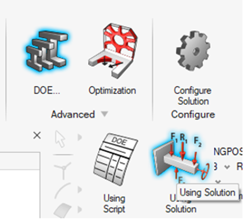
All input parameters and output results are already transferred to the optimizing tool.
You can select which parameters you want to keep and also define the ranging values.
You can also add the output you want to focus on: here output power and cross section of magnet.
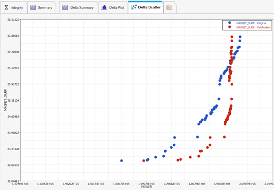
You can create DOE, fit function, optimize on fi functions and then recompute the Pareto plot with initial SimLab solver. You can see on the screenshot below that the difference between fit functions and real functions is less than 5%.
Conclusion
With this tutorial, you will learn how to set-up all these steps to become familiar with the concepts and the tools. You will find link to download the documents and the starting files.
With continued research and advancements in simulation capabilities, addressing optimization challenges will become more precise and efficient, ultimately benefiting industries reliant on high-performance magnetic materials.
Access
All files corresponding to this example are accessible in the following link:
2D_MT_DOEoptimPMmotor_SL2025.1.zip
Note :
The tutorial packaging may evolve with each new version, but not mandatory. The latest version of the tutorial package will automatically work with the most recent release of SimLab.
Example: After installing the SimLab 2025 release, you will find the latest Tuto_2024.zip package. This means that the tutorial has not been updated since 2024 release, that the tutorial does not need to be updated, and that the tutorial still works in 2024.1 release and 2025 release.
Step to follow:
- Follow the example step by step, the corresponding files are in the folder "Example_name_StepByStep" containing:
- Input folder: contains initial *.slb databases an other files needed to be able to play manually the tutorial by following the step by step document
- Output folder: empty (contains the obtained results after to play the tutorial)
- Tutorial folder: contains the document describing the example step by step
- To play the tutorial by scripts, the corresponding files are in the folder "Example_name_PlayScripts" containing:
- Input folder: contains initial *.slb databases an other files needed to be able to run scripts of the tutorial
- Output folder: empty (contains the obtained results after to play scripts of the tutorial)
- ScriptsTutorial folder: contains script files to be able to play each analysis
