The suspension system is one of the most important parts of the vehicles, which can
reduce the impact loads from the road to improve the automotive ride comfort and stability [1]. One of the very known and useful model to study the comfort and stability of the car is the
quarter car model suspension system, that consists of one-fourth of the car (one wheel). For sure some assumptions are adopted on that model, but that doesn't detract the numerous engineering applications using this
dynamic system. For those who are interested in
dynamic systems modelling, in this article I will discuss three different approaches demonstrating how useful the use of
numerical tools can be to solve them. To illustrate these methods, I will use a well-known model in the automotive world, which is the
quarter car model, and I'll show that is possible to
integrate all the solutions in a single platform. The approaches are:
- Signal-based diagram (Altair Activate)
- Physical block diagram (Modelica)
- 3D Multibody environment (Altair MotionView/Altair MotionSolve)
The starting point of modelling a dynamic system is understanding the bodies behavior (displacement, velocity, acceleration) that make up the system. To describe the model we usually study the degrees of freedom (from inertial and non-inertial axes) [2]. The system bodies and their connectors (rigid, springs, dampers) are isolated in order to uncouple the system and facilitate the modelling of each one individually, which after will be interconnected in order to represent the complete system. This is a very important task for the engineer, understand how the system works, and how it will be represented through differential equations (linear or non-linear). These equations will be the core for the system modelling, regardless the approach that will be used.
Quarter car - Dynamics of the model
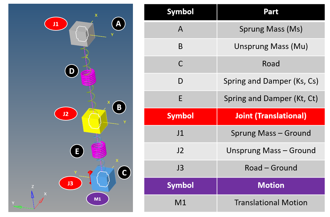
Quarter car system is a
two degree of freedom system, where there are
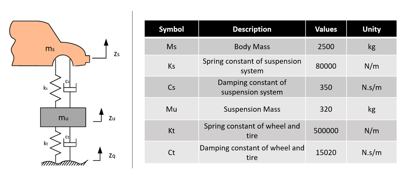
two bodies: Sprung (car) and Unsprung (suspension, wheel, tyre) mass. Although it is a simplified model,
stiffness and damping of the systems are used so as not to consider everything rigid (which is not representative in a physical model). Thus, between the road and the suspension, the stiffness and damping of the
tyre and wheel are considered, and between the suspension and the car, the stiffness and damping of the
spring and damper are considered. To validate the model some known parameters were used [3]. Highlighting that I've used a
passive system (without active actuators), check the figure below [1]:
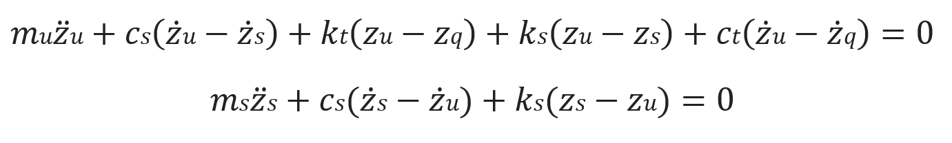
Where the differential equations of the system are (obtained by a free body diagram):
There are two second order equations where the initial conditions of each degree of freedom will be zero and the input will be
Zq once it is the
road displacement. For practical purposes I used a
Step Input, once the aim of this article is
demonstrate that is possible to model and solve the system using different approches. So basically each approach, regardless on its environment (0D, 1D or 3D)
will solve the differential equations above in order to obtain
Zs that is our desired varible (
car displacement), that further could be improved in order to provide comfort to the driver and passengers.
1. Signal-based diagram
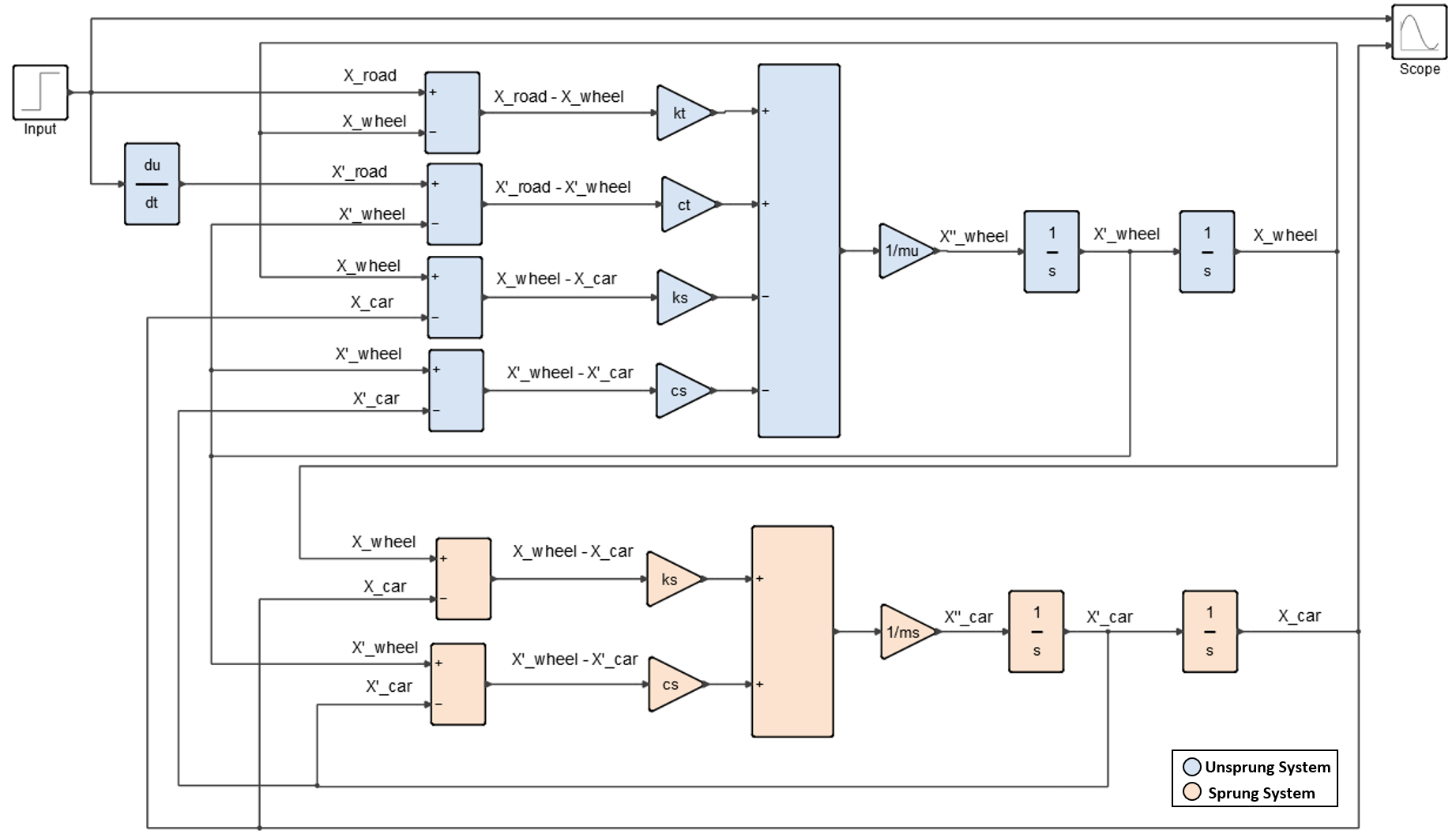
The strategy used to model in a 1D signal-based environment is
dividing the equations in terms, in order to insert them and at the end obtain the highest order variable (in this case the displacement of sprung and unsprung mass). It should be noted that it is a coupled system, since there are
dependent variables between them, so there is no way to solve them decoupled. But for the modeling, this is the easiest method to do. I usually start with the
largest sums in order to already get the
highest order variable and use them in the loops that generate the variable itself. This is a somewhat abstract method, but in a block diagram you should use the v
ariable that will be calculated to compose the previously equations. The block diagram of the quarter car system is shown below (remembering that the axis and signals of each variables depends on your free body diagram):
For sure I could use a
state-space block, including with this option you can solve using a
simple 0D script, or if you'd like to be deeper into the script, you could use the function
ode45, that is the Runge-Kutta method. but I have developed using
simple blocks to illustrate the more normal way to model this kind of system thinking of
1D signal-based.
2. Physical block diagram
Modelica is a non-proprietary, object-oriented, multi-domain modelling language for
component-oriented modelling of complex systems [4]. Users can represent
physical systems using simple blocks which already represent the
mathematical model, this way the blocks can be directly connected and their propertires can be easily set. There are several implemented blocks: Mechanical, electrical, hydraulic, thermal, control etc. Nowadays Modelica is integrated with Altair Activate so a
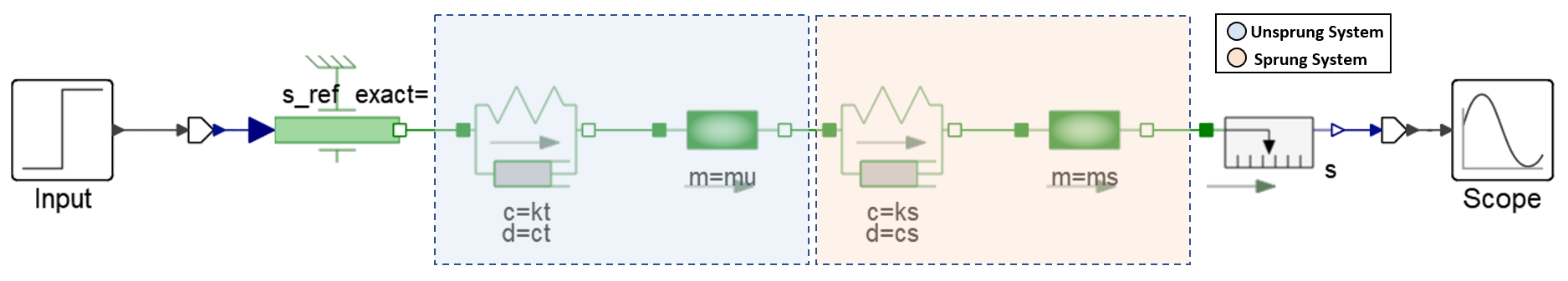
hybrid model (signal-based and physical blocks) can be implemented just using a simple "converter" block (represented below between the input and output blocks).
Its modelling is really simple and we just have to think on the
real physical model components. As can be seen on the above figure, it is exactly the horizontal representation of the first figure present on
Quarter car - Dynamics behind the model, just adding some blocks representing the
displacement input and
measurement (that is
our desired variable, Zs by the
equation).
3. 3D Multibody environment
The modelling of the 3D multibody system is very similar to modeling in Modelica environment in the sense that bodies, springs, dampers, inputs and outputs should be included. However, it should be noted that s
ome elements must be add and setups must be made in order to the
system works correctly. In 3D modelling there is a great freedom in the sense of setups, that is, each component initially has
6 degrees of freedom. In this sense, some
constraints (joints) must be add to provide to the components their correct degrees of freedom to work.
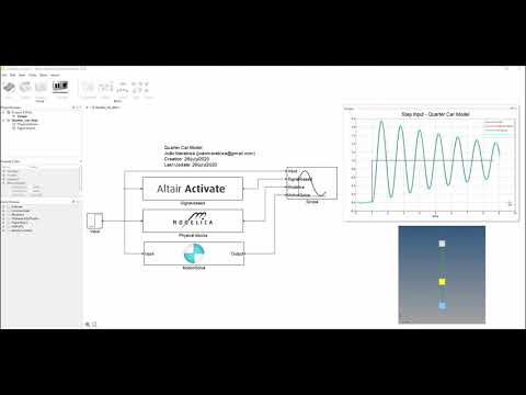
Results
Once all systems are modeled on their respective platforms, they can be integrated using Altair Activate. For this demonstration I have created 3 different blocks representing each one that I presented previously. On the right side of the video there is the result of each of them comparing with the desired input (step), there is also a visualization of the 3D model: As expected,
all the three results (Zs - car displacement) are basically the same, fulfilling what was proposed at the beginning of the article which is
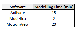
modelling and solve a dynamic system using different approaches. I know that engineers like and need metrics, so for curiosity's purposes I've created a comparative table with the time
it took me to model and setup each one of them completely after having the differential equations.
Remembering that this is just a
particular case of a specific system, and these are my particular consumption time and each professional has more aptitude in a specific type of modelling. The main point is to know that
all these solutions are available together and the engineer can choose the one that will be the most useful for his/her day-to-day work.
References: - Zhou, C.; Liu, X.; Chen, W.; Xu, F.; Cao, B. Optimal Sliding Mode Control for an Active Suspension System Based on a Genetic Algorithm. Algorithms 2018, 11, 205.
- https://altairuniversity.com/44492-modeling-and-control-a-ball-beam-system-mbs-1d-co-simulation/
- http://ctms.engin.umich.edu/CTMS/index.php?example=Suspension§ion=SimulinkModeling#1
- https://www.modelon.com/what-is-modelica/