Overview
The antenna reciprocity theorem [1] relates the antenna load current for given plane wave excitation to the radiation pattern when the antenna is excited. The antenna is assumed to be made of linear and reciprocal components.
With the CADFEKO Reciprocal Excitation solution configuration, the antenna load response under plane wave excitation can be computed as a post-processing step in POSTFEKO.
Using this workflow reduces computationally effort as only the antenna under a single excitation needs to be solved. For example, modelling a direction-finding antenna array with multiple plane wave incidence angles reduces the number of solutions to the number of antennas in the array times the number of frequencies. In post-processing the user can specify the plane wave properties like amplitude, polarisation, polarisation angle and ellipticity. The incident plane wave directions will either coincide with the discrete samples of the requested far field pattern or could be specified when a continuous far field request is available.
This workflow also allows calculation of induced currents and voltages of cable harness loads, with plane wave excitation and Schematic link connections. Schematic link connections are only supported for radiating cable harnesses.
CADFEKO solution setup
New Reciprocal Excitation configuration
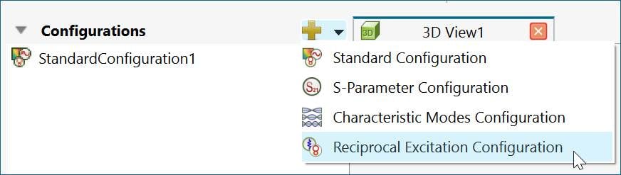
Figure 1: Reciprocal Excitation solution configuration
Two parts of the Reciprocal Excitation configuration:
1) Define loads where induced current with plane wave excitation is required.
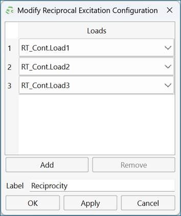
Figure 2: Example of Reciprocal Excitation dialog
2) Add far field request(s). Two options: discrete far field sampling or continuous far field. First choice would be to request a continuous far field as then the user can specify arbitrary plane wave incident directions as part of the POSTFEKO post processing step. However, the continuous far field request is not supported or efficient for all solution options, like real ground planes and electrically large structures. In these cases, it is recommended to request a far field with discrete sampling, and the plane wave incident directions will be limited to the discrete sampling of the far field.
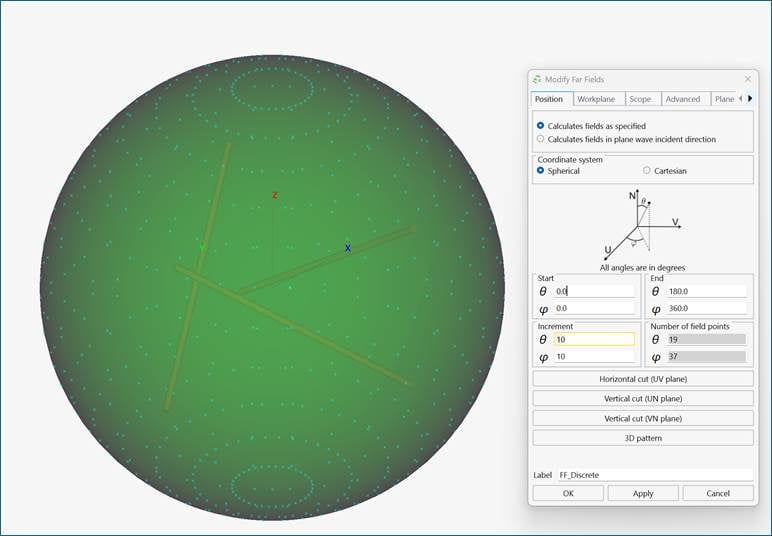
Figure 3: Example of far field request
POSTFEKO post-processing
1) Load the solved model containing a Reciprocal Excitation configuration
2) Run the Reciprocal Configuration application macro.
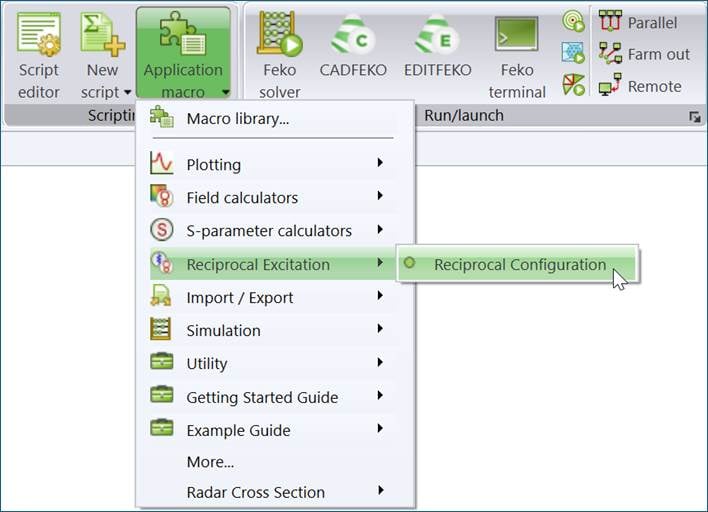
Figure 4: Reciprocal Excitation post processing application macro
3) Select a far field associated with a Reciprocal Excitation configuration
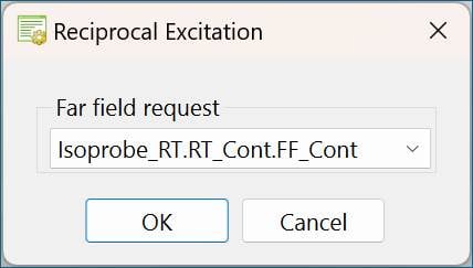
Figure 5: Dialog to select far field request associated with Reciprocal Excitation configuration
4) Specify solution properties: Frequency solution and plane wave properties
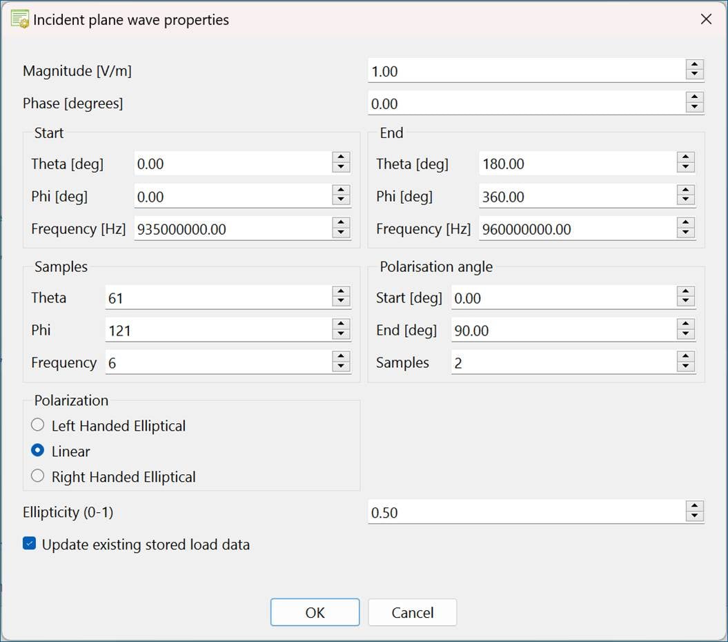
Figure 6: Dialog to set frequency and plane wave solution properties when both continuous frequency solution and continuous far field request are selected
For both continuous frequency and a continuous far field request all parts of the dialog are active, see Figure 6. For continuous frequency and a discrete far field request the plane wave incident angles are greyed out (can’t be changed), see Figure 7.
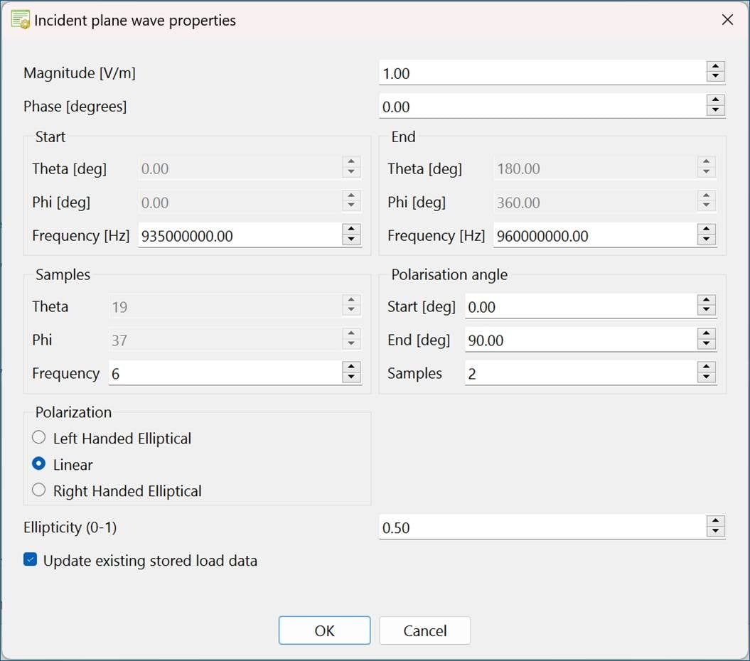
Figure 7: Dialog to set frequency solution properties with continuous frequency solution and discrete far field request are selected
5) OK to run the application macro
6) The induced load data is stored with the same label as specified for the Reciprocal Excitation configuration, see Figure 2. Hovering the mouse pointer over the stored data item listed in the Project browser will provide more information associated with the induced load data, see Figure 8.
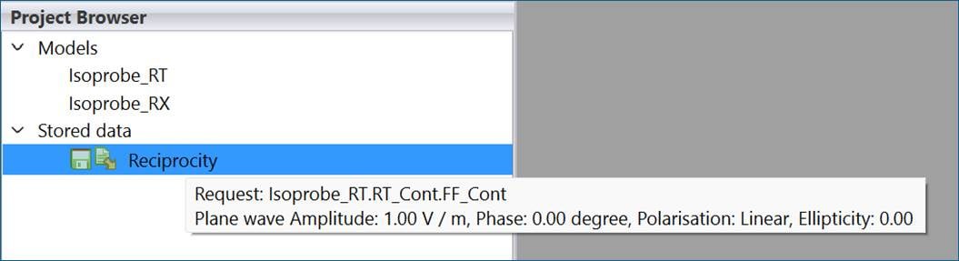
Figure 8: Stored data note
7) The stored data has 5 axes: Loads, Polarisation, Frequency, Plane Wave Theta and Plane Wave Phi and can be plotted on Cartesian graphs and Cartesian Surface graphs. The normal load quantities are available: Current, Voltage, Impedance and Power, see Figure 9 for example of load power vs incident plane wave phi angle.
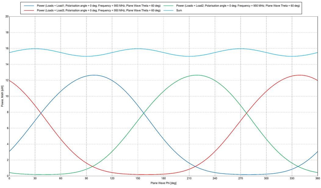
Figure 9: Example of load power versus plane wave phi
8) The stored data can be exported to file via the Project browser
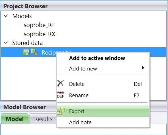
Figure 10: Export stored load data
[1] R.H. Clarke and John Brown, Diffraction Theory and Antennas, Ellis Horwood Series in Electrical and Electronic Engineering, 1980.
