This document aims to introduce the various ways one can study buckling behavior in S-FRAME. We will examine this using a generic steel girder bridge structure, which has been deliberately altered to weaken it, hence allowing us to illustrate buckling behavior.
The modifications from the original design include:
- Reduction of span lengths, and simplified geometry
- Modification of girder section dimensions
- Simplifications of the loading (only self-weight and 60 PSF dead load on top of girder flanges considered).
- Girders are assumed to be continuous, and no expansion joints were considered.
- Pin-Roller-Pin support conditions on bottom flanges of girders.
- Truss Framing is integrated into webs/flanges at discrete points along the girder.
- Ignored the stiffness of bridge deck.
- Geometry perturbations were hypothetical scenarios, purely for illustration.
For these reasons, it is safe to assume that this model does not represent any real-world structure, and the objective of this exercise is to review potential buckling behaviour on a fictional structure.
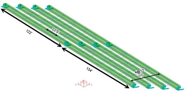
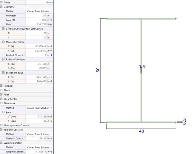
The model has four girders spaced twelve feet apart, with a truss structure providing lateral stability at a typical twenty two ft spacing. The bridge structure has two spans, each simply supported. One span is one hundred thirty four ft long, and the other is one hundred twenty two ft long. The girder cross section is a wide-flange shape that has a flange width of forty inches, and a depth of sixty inches, and flange/web thickness of one half of an inch. We recognize that this section size may not be realistic, but it will allow us to illustrate buckling behavior.
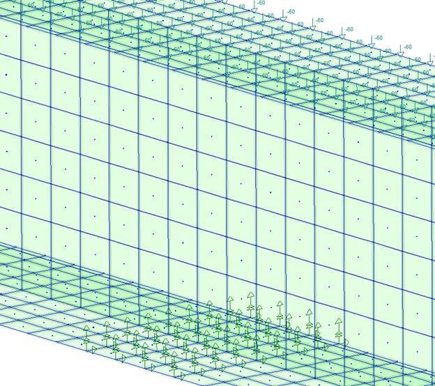
This model will be subjected to the steel girder’s self-weight, and a dead load of 60 lb/ft2 applied to the top flange.
We will start by running an Unstressed Vibration Analysis. This is a free vibration analysis, examining the dynamic characteristics of the model in the absence of any damping or loading. We will include the impact of self-weight and applied dead loads on the inertia properties of the bridge in the mass matrix of the structure. The mode shapes and associated natural frequencies/periods can be a helpful way to validate our structure and predict structural behaviour. From this first mode, we can see that 21.5% of the structure’s mass is participating in the X-direction for this mode shape and has a return period of 0.827seconds.
Next, we run a Linear Static Analysis. This will examine the behaviour of our steel girder structure with the assumption that the material and geometry behave in a linear manner, and the loads are applied as static loads, all at once.

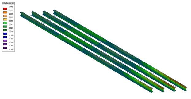
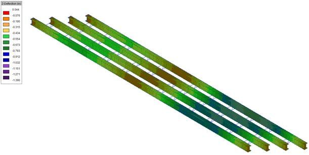
As we can see from the above plots the maximum vertical deformation occurs, unsurprisingly in the 134’ span, reaching 1.377 inches in the Z-axis. Interestingly, we also observe some lateral deformations due to the vertical Self-Weight + Dead Loads. Note that there are minor geometric discrepancies in overall span length between the girders such that the girder on the right side of the above image was slightly longer than the others, causing a slight asymmetric stiffness.
Next, we run a P-Delta Static Analysis. This analysis will consider the stressed state of the model. A P-Delta Static Analysis is a two-step process. First, the solver will perform a linear static analysis and compute the stress-stiffness matrices for the structural elements in the model. The next step involves a second linear static analysis, this time with the updated global stiffness matrix. If the loading approaches or exceeds the structure's buckling capacity, we generally expect discrepancies between the results from Linear and P-Delta Static Analyses, such as increased displacements.
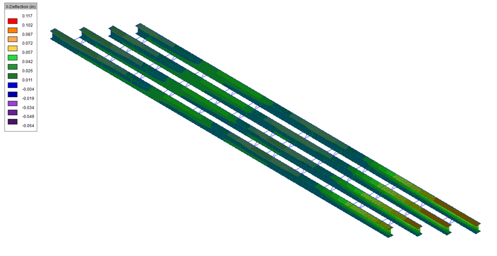
As we can see the maximum vertical deformation is similar between Linear Static (-1.377”) and P-Delta Static (-1.380”) analysis, which is likely an indication that the model under its current loading is not close to its buckling limit. A similar trend is noticed with the lateral deformation, with linear static analysis yielding a maximum of 0.116”, and P-delta static analysis coming to 0.117”.
What Have We Learned: The main takeaway from these simulations is that our loading may be too low to induce buckling. These preliminary analyses can also help us better understand the high-level structural behaviour before we perform more rigorous analysis.
Let us now try to predict a load that could lead to buckling. We'll look at a few different methods for doing so, starting with a P-Delta Buckling Analysis. A P-Delta Buckling Analysis computes the so-called buckling load factor, which, if used to scale the load case or load combination under investigation, will cause buckling.
A buckling load factor less than or equal to 1.0 implies that the load case or load combination under investigation will cause buckling. In other words, we must strengthen the structure's design to avoid the potential for a catastrophic failure. Ideally, we want to see buckling load factors much greater than 1.0. How much greater? That's up to you to determine.
For our model, we will investigate the “Dead + Self Weight” Load Combination.
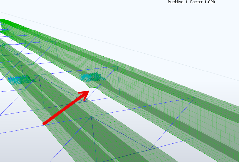
From the above screenshot, we can see that we are getting a mode shape for our buckling analysis showing buckling on the lower flange near a support at a buckling load factor of 1.82. This means that we would need to increase the magnitude of the “Dead + Self-Weight” load combination by a factor of 1.82 to cause the model to buckle as such.
What Have We Learned: If we increase the magnitude of the “Dead + Self Weight” Load Combination by a factor of 1.82, we will reach the structure’s Euler Buckling Limit.
It’s worth noting that both the P-Delta Static Analysis and the P-Delta Buckling Analysis use the original geometry of the structure; in other words, they do not update the geometry to reflect displacement under loading. This limitation is acceptable as long as displacements and deformations remain small, which is usually the case with the type of structures structural engineers deal with. However, as we approach buckling conditions, this assumption no longer holds, and one must rely on a Nonlinear Static Incremental Analysis. We will attempt this next with 30 load increments, and we will include incremental results in the analysis output. The nonlinear static analysis works by dividing the load vector into equal increments (in our case, 30) and solving them incrementally. The starting point for each successive load increment is the solution (i.e., the deflected and stressed state of the structure) of the previous load increment, and the analysis will proceed until all load increments are solved. It is worth noting that increasing the number of load increments can be beneficial in improving accuracy, particularly when the behaviour becomes more ‘nonlinear’. Another advantage is that it improves the granularity of the results, which can be helpful when observing the onset of buckling.
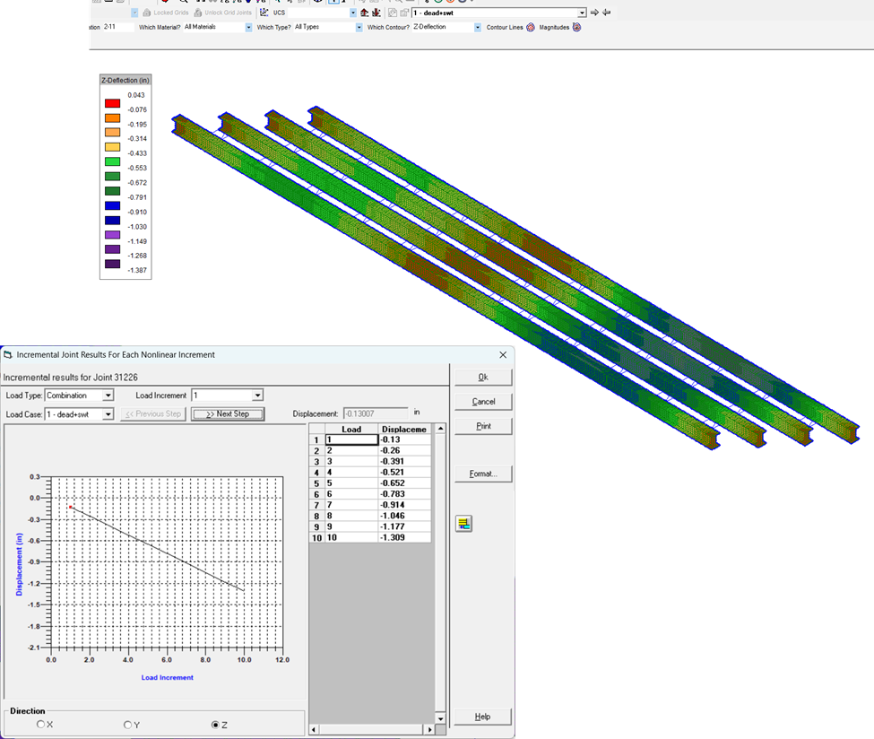
From the results shown above, the maximum vertical deflection is -1.387 inches, which falls between the Linear and P-Delta Static Analysis results described earlier. This could be a scenario where the deflected shape’s behavior influences the results, albeit in a minor way. We have also included a screenshot of the incremental results for a reference joint in our model, showing the Z-displacement versus the load increment. As shown in this plot, the results are linear. For a nonlinear static analysis, the buckling behavior must be interpreted through a careful study of the sequence of results. We classify buckling as the point at which our structure experiences a sharp increase in the deformation from a slight increase in the applied load. Clearly, there is no evidence of buckling under the “Dead + Self-Weight” load combination.
What Have We Learned: The P-Delta Static, P-Delta Buckling and Nonlinear Static analyses do not predict buckling under the “Dead + Self Weight” Load Combination.
Continuing our investigation using the Nonlinear Static analysis, we scale the "Dead + Self-Weight" load combination to determine how close it is to a buckling load. We'll scale it by a factor of 8. When we increase the actual load conditions by an arbitrary factor, we should be prepared to receive warning and error messages from the solver (like in the image below), and at some point, even a solver crash - these are actually giving us a clear indication of the onset of buckling.
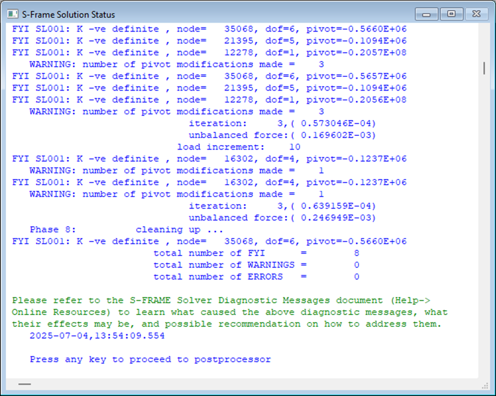
So, despite the presence of these Solver Diagnostic Messages, we use the incremental results, especially animations of the displacement history, to study the behaviour before and up until the point of instability.
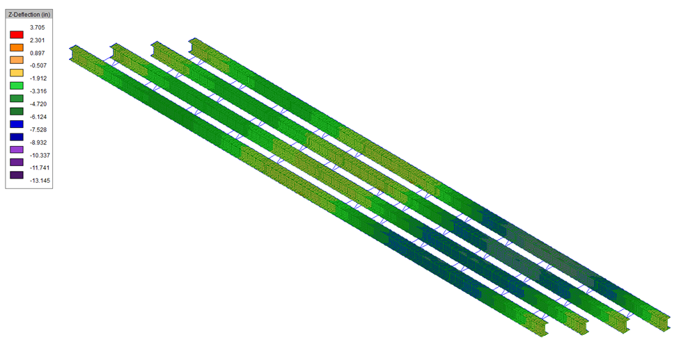
When reviewing the vertical deformations, we can see the maximum has increased by a factor of approximately 9.6, despite only increasing the loads by a factor of 8. This indicates the deformation vs. load plot is no longer linear.
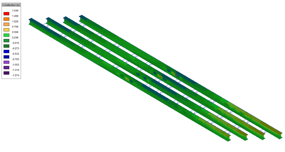
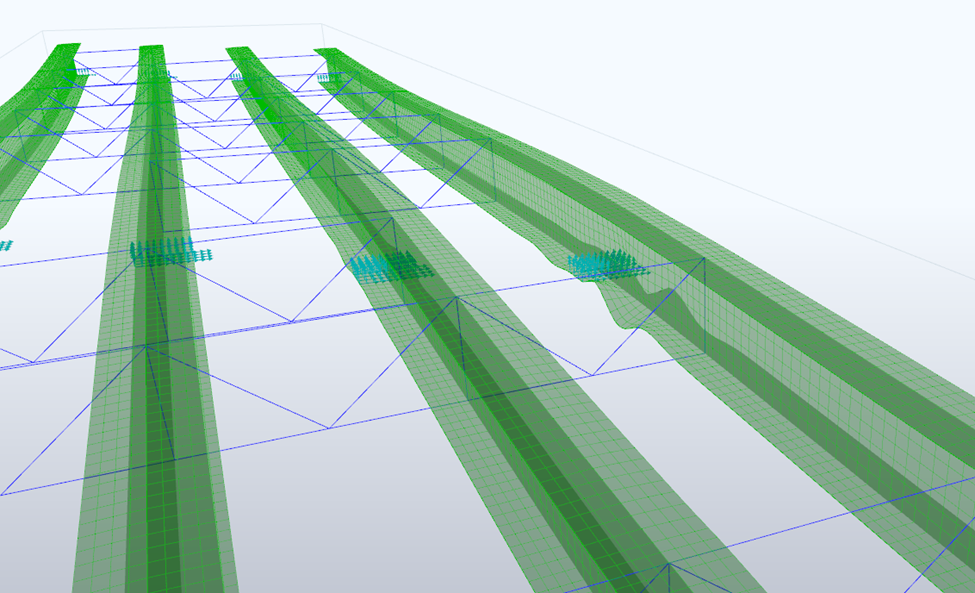
Further to the vertical deformation, we are also seeing some interesting lateral deformation, specifically concentrated near our interior supports.
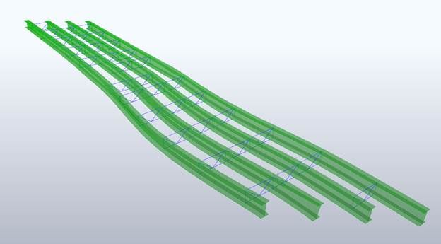
When we render the incremental deformation in S-VIEW, we can see a similar looking buckling observation to what was observed in the P-Delta buckling analysis.
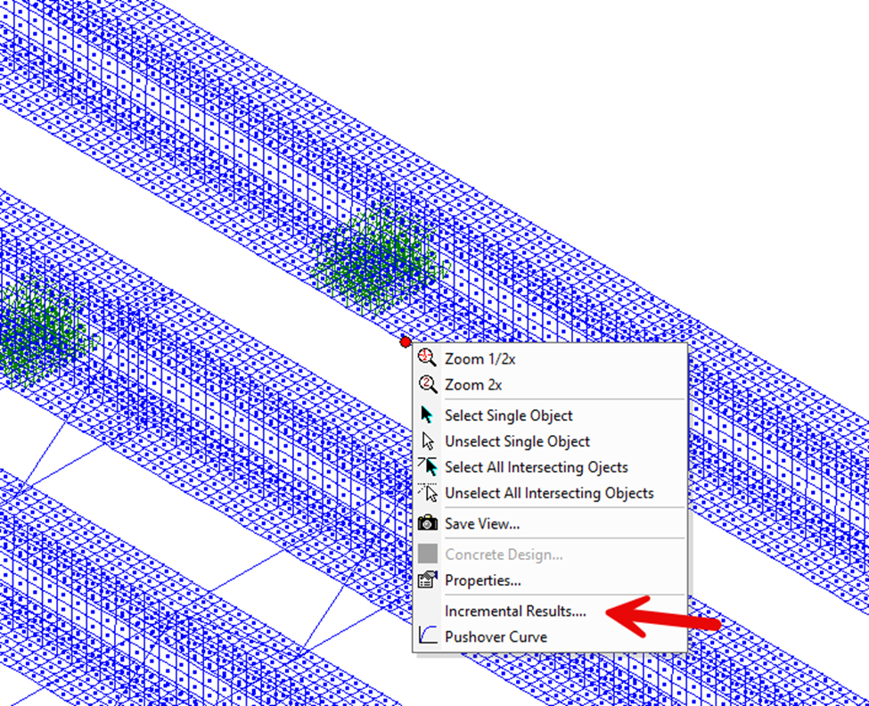
To study this in more detail, we can right click on any joint in our model and view Incremental Results.
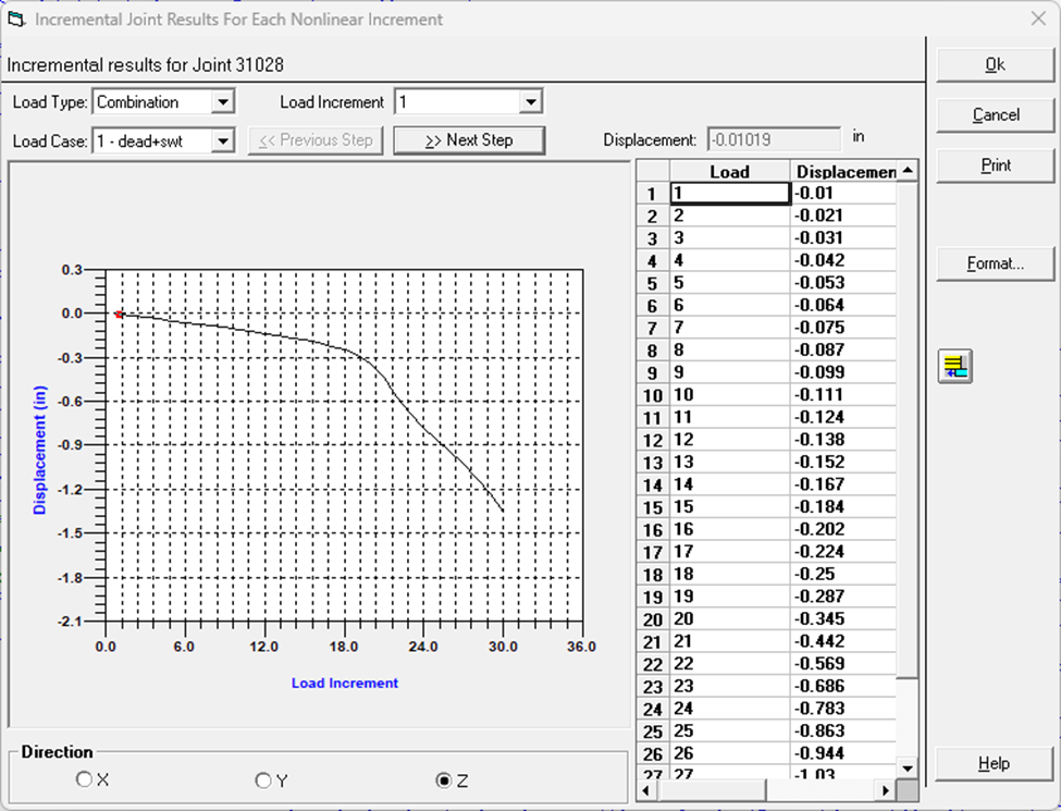
From this plot of the Load Increment vs. Displacement in the Z axis, it appears that buckling is occurring around load increment 19, when there is an abrupt deviation from the almost linear response. Remember that we increased the magnitude of our applied loading by a factor of 8, so this observed “buckling factor” would be approximately:

Therefore, we can say that from a nonlinear static analysis, we observed the sharp increase in deformation at approximately 5.0x the original load magnitude.
It’s worth noting that our analysis model does have some asymmetry due to the angled nature of the girder layouts/supports, etc. but is otherwise idealized to have ‘perfect’ geometry.
What Have We Learned: The Nonlinear Static analyses, an inherently more accurate analysis type than the P-Delta types, predicts that buckling will occur at approximately 5x of the “Dead + Self Weight” Load Combination.
For Part 2, see here:
