Authors: Ambrish Singh and Spyridon Mallios
1.0 Introduction
A Discrete Element Method (DEM) simulation can provide critical insights into the behavior of granular media subjected to various environmental, process, and operating conditions. However, prior to modeling process of interest, ensuring that the DEM simulation accurately captures the bulk material behavior is critical. This is achieved by material model calibration.
Consider the example of a Uniaxial Compression Test (UCT). The response of interest is the evolution of strain vs. stress during compaction and unloading.
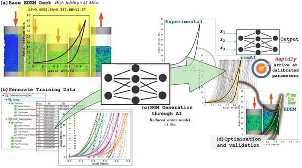
Using the material interaction and contact model parameters (EEPA), one must aim to capture this response in the simulation. The iterative nature of the calibration process makes it computationally expensive and slow. Using Altair's romAI, a significant speed-up can be achieved with a more comprehensive parameter sweep, allowing for an improved calibration workflow. This higher computation speed is attributable to the data-driven approach of romAI rather than EDEM's physics-driven approach. This workflow, as outlined in Figure 1, becomes progressively more effective when multiple bulk materials are to be calibrated against several experimental responses.
|
|---|
Figure 1: Workflow of efficient material model calibration using romAI |
Through Altair's romAI and HyperStudy (HST), the following methodology was implemented to simplify this process and rapidly arrive at calibrated parameters.
- First, using HyperStudy, a Design of Experiments (DOE) is created with a select set of material interaction and contact model parameters.
- The response of the EDEM runs, which in this case is the temporal evolution of stress and strain curves for each combination of Static Friction (SF), Plasticity Ratio (PR), and Bond Number (BN), is recorded in a CSV file. This data is subsequently used to train a romAI model.
- This 'trained' romAI model is later leveraged through HST to arrive at model parameters for an unfamiliar stress-strain response.
- The simulation files and other resources used in this article can be downloaded below
2.0 Generation of Training Data
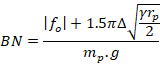
Uniaxial compression test within EDEM's Calibration kit with HST was leveraged to generate training and test data for the romAI model. Figure 2 shows the DOE scheme, through which the relationship between three inputs, SF, PR, and BN, and their effect on the strain-stress response of the numerical sample was explored. The following are some relevant considerations.
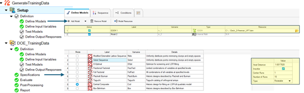
- The Bond Number is a derived quantity within the EEPA model. The following equation was used for its computation. The variation in BN is made through a change in surface energy and pull-off force in a proportionate amount.
2. The result from the unconfined compression is not included as part of this study.
3. The DOE follows a Rotatable Central Composite Design scheme. This generates 15 data points within the parameter space, as shown in Figure 2.
|
|---|
Figure 2: (a) Rotatable central composite design for generation of training data, (b) strain-stress response for various combinations of input variables, and (c) bounds of input variables |
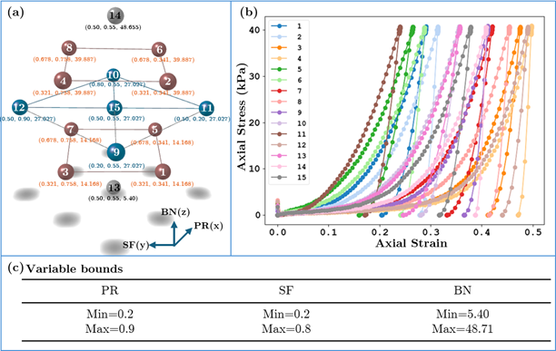
The workflow for data generation can be streamlined through HyperStudy. As shown in Figure 3, first, the model is defined by pointing HST to the UCT calibration deck. Next relevant inputs and responses are defined. A DOE is added, taking its definition from the setup, and EDEM is iteratively run, generating training data. Purge functionality of HST is implemented to delete all the 'h5' files except '0.h5'. This ensures minimal consumption of memory.
|
|---|
Figure 3: Use of HST to generate synthetic training data |
|
|---|
Media 1: Workflow demonstrating the use of HyperStudy for the automated generation of synthetic training data |
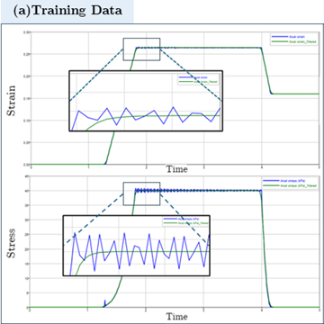
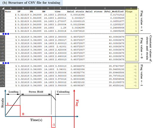
After executing all 15 EDEM runs, the generated data is to be compiled into a single CSV file. Figure 4 shows the structure of this compiled CSV file. The variable values remain constant for each segment and are repeated across all the rows, whereas the stress-strain response evolves over time and is recorded till the end of each simulation.
For optimal performance of the romAI model during training and later testing, the training data were prepped with the following operations.
A filter of 5Hz was applied to the strain and stress responses of each segment to eliminate noise from the dataset. Observing the plots for strain and stress responses reveals noise in the data from the peak of compression and throughout its duration. This noise can be partially attributed to the force controller within EDEM attempting to hold the pre-defined level of compression stress before unloading. Figure 4 shows the filtered and original values for one segment.
After filtering, an additional column, called 'Flags', was added. This column was populated with row values of '1' for the loading part, '0' for the stabilization part, and '-1' for the unloading part. The flag column helps identify the three phases of the uniaxial compression test for each segment.
|
|---|
|
Figure 4: (a) Use of data filter in romAI director (b) Structure of compiled CSV file. The CSV file contains 15 segments from the DOE runs |
3. Constructing romAI Model
Constructing a romAI model starts by importing the prepped training data into the romAI director. A static model is constructed, implying that inputs and outputs are defined; however, no system state is specified. Four inputs: SF, PR, BN, Strain, and Flags are specified, and the stress value is considered as an output.
'Auto exploration' and 'Check Points' functionality of romAI can be leveraged for the selection of hyperparameters. An excellent agreement between the romAI predictions against the training data can be observed in Media 2.
|
|---|
Media 2: Training and testing (against training data) of romAI model |
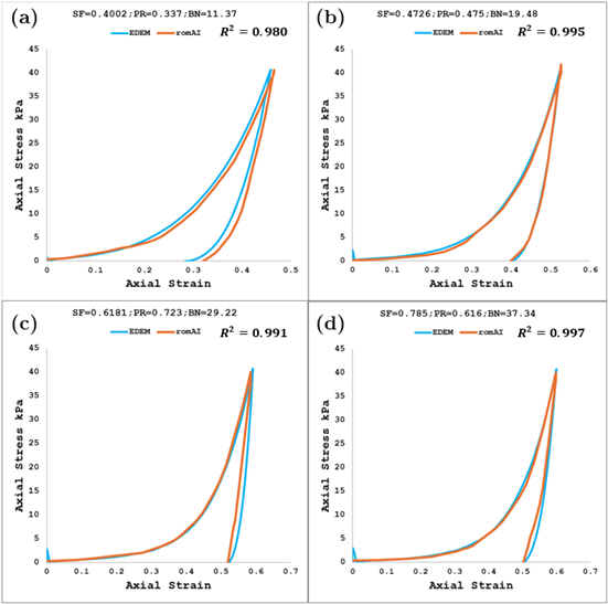
Four sets of input variables, which were foreign to the romAI training data, are used for testing the model. Figure 5 shows the performance of the romAI model against the EDEM results for test parameters. An excellent agreement between the two suggests that the romAI model is sufficiently trained with the right set of hyperparameters and is now fit to be used for calibration, substituting EDEM.
|
|---|
Figure 5: Comparison of romAI results against EDEM results for four sets of test variables. These input variables were excluded from the training data of the romAI model. An excellent agreement can be seen between the two (EDEM and romAI) models. |
4. Twin Activate Model Setup
Up to this point, the trained romAI model requires 5 Inputs to be evaluated: the 3 material properties, the Flag, and the Axial strain value. Before we can use this model for calibration purposes, we need to format and structure it in a way that only the 3 material parameters are needed as inputs. To do this, we leverage Altair Twin Activate, a Math & Systems-focused software.
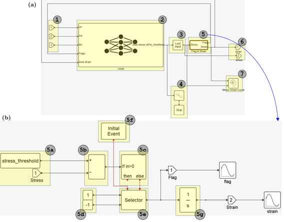
More specifically, we use Twin Activate to integrate the romAI model and internally compute the Flag and Axial Strain values based on the progress of the simulation. These two are computed via a combination of Mathematical modeling & Activation Operations, as shown in Figure 6.
The Flag variable starts from a value of 1 (as we always start the test with the compression phase) and switches to -1 when the "stress threshold" is reached. In parallel, Axial Strain is computed using the Flag's value integral over time. As a result, the Axial Strain is increased until the "stress threshold" has been reached and then decreases linearly over time. The simulation is terminated using a "Stop" block when the Axial Strain reaches the value of 0. To avoid an algebraic loop, a "Last Input" block is used, since the output of the romAI model is required to calculate the Flag & Strain inputs.
|
|---|
Figure 6: romAI deployment in Twin Activate |
5. Optimization using the Twin Activate-HST workflow
The Twin Activate model, which contains the trained romAI block, can be executed through HST. The advantage of this workflow is the smart automation offered by HST in job/ run management. Additionally, HST has several optimization and post-processing tools that can be leveraged for an intelligent sweep of the parameter space. The Activate file, with the extension '.scm', can be brought inside the setup definition of HST with access to input variables and output responses. The optimization/calibration objective is defined as follows.
- Minimize the difference between experimental and romAI results for the stress curve by optimal selection of input variables (within specified bounds)
- Minimize the difference between experimental and romAI results for the strain curve by optimal selection of input variables (within specified bounds)
Media 3 outlines the workflow for achieving this optimization. A Python script that uses interpolation to ensure that the experimental data and the romAI outputs are of equal length is also added to HST.
A guide to preparing Twin Activate models for use in HyperStudy can be found here.
|
|---|
Media 3: Workflow for using the Activate model with HST for efficient material model calibration |
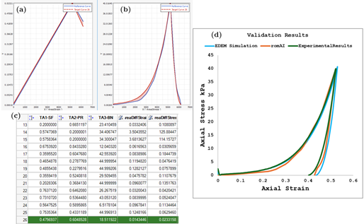
Once HST suggests the set of parameters that accomplish the set objectives, the next step is to test the results. This is done by running an EDEM simulation at the suggested parameters and comparing the EDEM's response with the experimental values. Figure 7 shows the comparison between the three sets of data. It can be observed that all three, i.e., experimental, romAI, and EDEM results, agree with each other within a reasonable margin of error.
|
|---|
Figure 7: Arriving at calibrated parameters by matching the stress-strain response of the romAI prediction to experimental results, followed by validation through EDEM simulation at the romAI predicted optimal values (highlighted in green) |
Further reading and references
