The Siemens Community Catalyst program was co-created with our community to acknowledge technology leaders who consistently contribute to the Siemens Community. Nominations are accepted on a rolling basis.
Dear all,
I have an exercise which I would like to extract near field from a horn antenna and import to another simulation (all in FEKO platform), then there is a weird result shown in the video as below link I just uploaded:
https://drive.google.com/file/d/1-NGAV75rxH2zKfahMF4qN6I2l8BpKN8c/view?usp=sharing
You can see the far field pattern with near field source I imported is completely opposite to original one. I would appreciate if anyone can show me how to simulate correctly.
BR/Marcus
Hi @Marcus Chang,
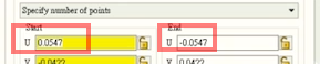
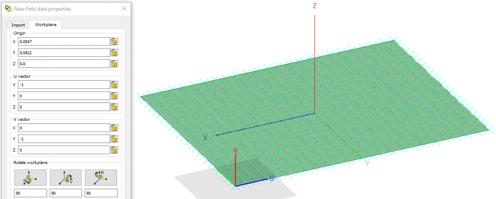
In the model where the near field is requested, the Start and End values of U are defined from positive to negative:
Therefore when trying to use as near field source, you should rotate the workplane of the source (or of the field data) so that the orientation agrees with the original model.
Hi @Torben Voigt,
Thanks for you immediately support, and it works now.
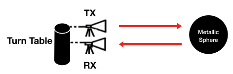
Here is another question for another exercise, I would like to use a horn antenna to radiate on a metallic sphere, then try to use the same horn antenna to receive power reflected from the metallic sphere.
First, I extract near field data from a horn antenna I just run (please check file named horn_X band_190309.cfs).
Then in simulation 1 (please check file named FF source_PEC.......cfs), I use this near field source as TX and radiate to a metallic sphere, then I can get the results of the near field from a surface of sphere, and extract its as the near field source for simulation 2 (please check file named temp_190313.cfs)
In simulation 2, I use the near field source from previous results (on surface of sphere) and radiate to a near field receiving antenna (the same horn antenna) and try to get the result that how much power it can receive.
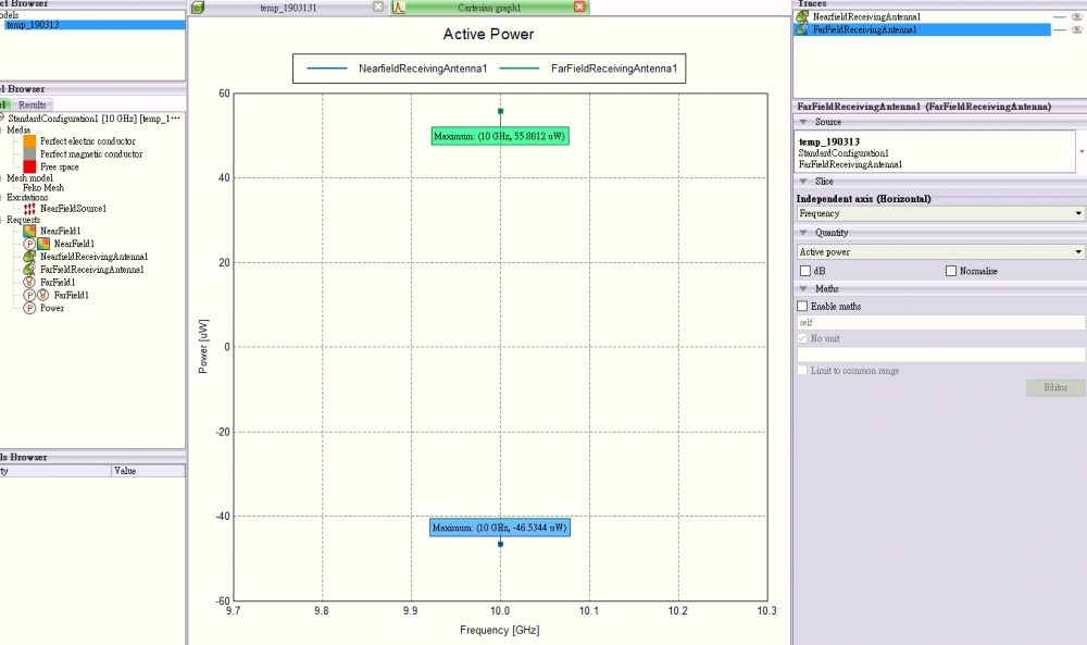
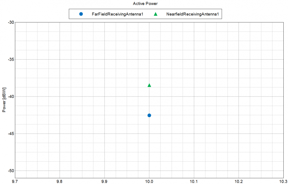
However, I get two different results from different method, one is using far field receiving antenna, another one is near field receiving antenna as below.
And also, it is weird that the power is negative, could you please help us check again what's happening to this simulation?
And the last question is, how could we get results of the far field pattern from receiving antenna, not just power calculation?
onlyonechancy@gmail.com
I would need the *.cfx files to investigate.
I already update attached file as below, please check it.
Let check what you did:
The three new model files are attached:
Thanks for you support.
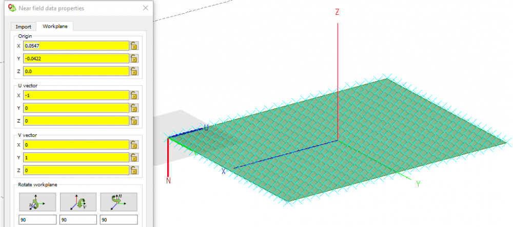
About Mistake #2, the location of receiving antenna (RX) should be the same as transmitting antenna (TX).
So I place the near field data at z=0 rather than z=0.2138m. (horn aperture is placed at z=0).
Then I increase the distance between horn and metallic sphere to 72 times lengths of wavelength. (2*D^2/lambda=72 lambda) to satisfy far filed requirement, so that warning 39270 is not shown again.
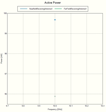
Finally I can get the results shown as below, please check:
But... this results do not accord with the number calculated by MATLAB, the coding is shown as below, please check:
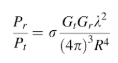
f=10*10^9;c0=3*10^8;lambda=c0/f; %units: m lambdaPt=1;Gt=18.3; % simulated in FEKOGr=18.3; % simulated in FEKOr=3*lambda %units: m, radius for metallic sphereRCS=pi*r^2R=72*lambda %units: m, distance between sensor and objectPr=Pt*1*Gt*Gr*RCS*(lambda^2)/((4*pi*R^2)*(4*pi*R^2)*(4*pi))
so that I can get Pr=177.56e-09 (W), 177nW approximately, almost twice the power of the results (100nW) simulated in FEKO.
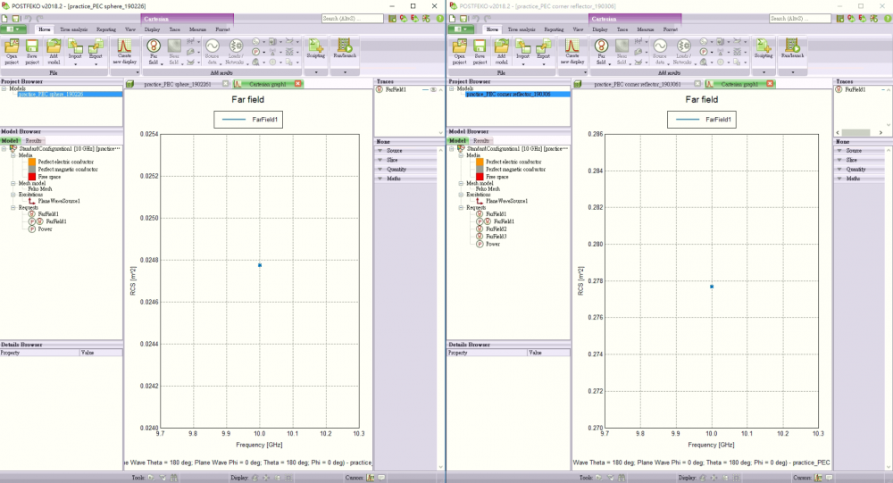
Second question is, is it possible to get far field pattern of the reflected field of sphere?
Unfortunately I'm not sure about the Matlab code. Maybe someone else (@mel, @JIF) could have a look?
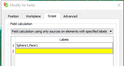
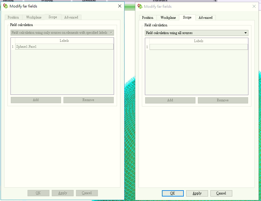
You can get the far field pattern of the reflected field of sphere by doing this:
This will then only use the contribution of the surface currents of the sphere.
Dear @Torben Voigt @mel @JIF
MATLAB code is just a easy way to calculate it.
But it is a simple and fundamental formula as below:
while the RCS value I use is:
here Gt=18.3=Gr, lambda=0.03(m), r=3*lambda, R=72*lambda (=2D^2/lambda, D=2*r) and Pt=1W (in Feko),
then I can get the value of Pr is equal to 177nW, however, the results simulated in Feko is less than 100 nW.
And thanks again for your suggestion of receiving far field pattern of reflected signal, I will try it and get back to you if there is any further questions.
Dear @Torben Voigt,
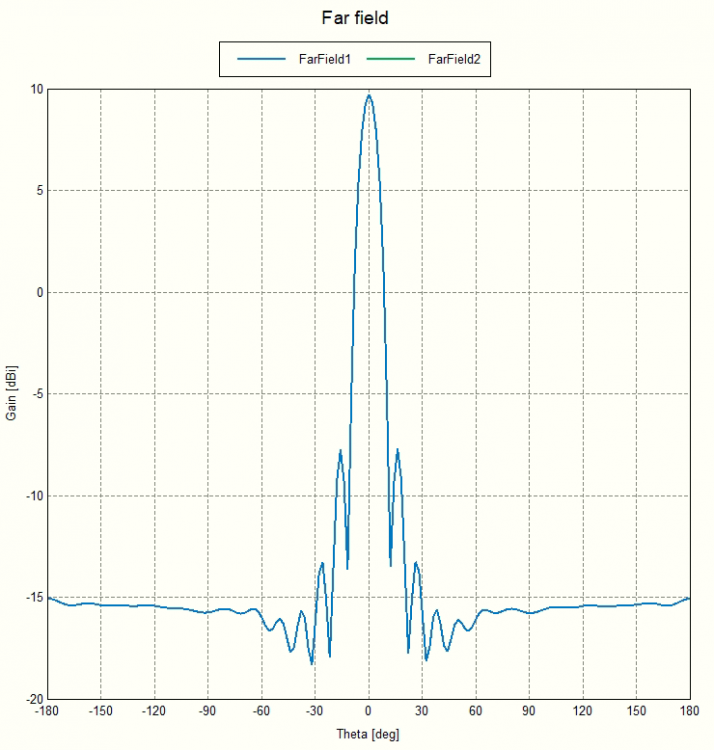
For the suggestion of the contribution of the surface currents of the sphere you provided, it seemed not work as below,
there is no differences when I use it, please check:
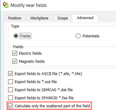
If you get identical far field results for both, then I assume you have in addition 'Calculate only the scattered part of the field' activated:
This will in this model of course give the same results, as the sphere is the only scattering object. So, in both cases you will get the scattered field from the sphere surface.
Dear @Torben Voigt @mel @JIF,
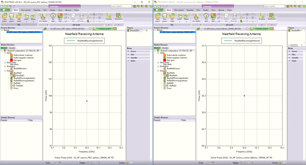
Recently, I try to run some simulations for metallic sphere and corner reflector respectively, the results for these simulation is weird, the received power bounced by metallic sphere is larger than corner reflector.
But actually, the RCS for metallic sphere should almost 10 times smaller than corner reflector, no matter it's calculated by formula or simulated in FEKO (I also upload these simulations as attached, please check)
So I would like to check with you again, to see what's happened to the setting in FEKO.
For the corner reflector you're using PO, but with PO no multi-reflections between PO faces are taken into account. A corner reflector is THE classical example where PO is not feasible. Furthermore, the asymptotic methods (PO, LE-PO, RL-GO and UTD) are only feasible if the model is electrically very large, e.g. 20 lambda, bigger is better, but the corner reflector is only around 4 lambda. You should definitele use MoM / MLFMM here. Same goes for the sphere, which is only 3 lambda in radius.
When calculating the scattered field of the reflector and the sphere correctly (MoM), the received power of the reflector is around 10 times higher than that of the sphere.
It works now, the received power for RX antenna in situation of corner reflector is also 10 times larger than metallic sphere.
Thanks for your suggestion!
If I would like to do multi-frequencies simulation, such as with a bandwidth, how to use script to import near field data for every single frequency in this case.
Because when I try to run a multi-frequencies problem, I use the first .cfx file and add multi-frequencies setup, I can get a NF data with multi-frequencies.
But when I use this NF data as my equivalent source (NF source), the error message was shown as below:
ERROR 3392: The near field source cannot be used inside an implicit frequency loop (frequency dependent data)
And I check there was a member had similar problem, it seemed like I need to solve it with EDITFEKO.
Can you provide us an example (EDITFEKO), for this three files, such as how to write a loop then I can finally get a plot with RCS values in a bandwidth, such as 9-11 GHz.
It's not necessary to use EDITFEKO for this anymore. In principle you need one configuration per frequency. Also you need one Field data per configuration. Please have a look at the attached CADFEKO script.
It was all created using Macro recording and a little editing. You can use it and fit it to your model.
Open base_model.cfx and run the script from there, it should give you some insight in the process.
Due the the version problem, could you please help us provide the modified file in previous version (2018.2-338937 (x64)) in this transition period?
Here you go:
Please install FEKO 2019 soon. It's hard to provide support for different versions.
Here is another question for scripting related to this case.
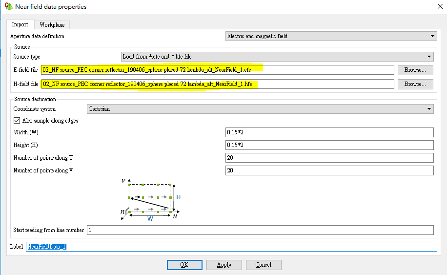
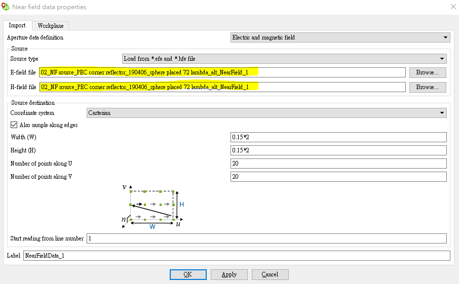
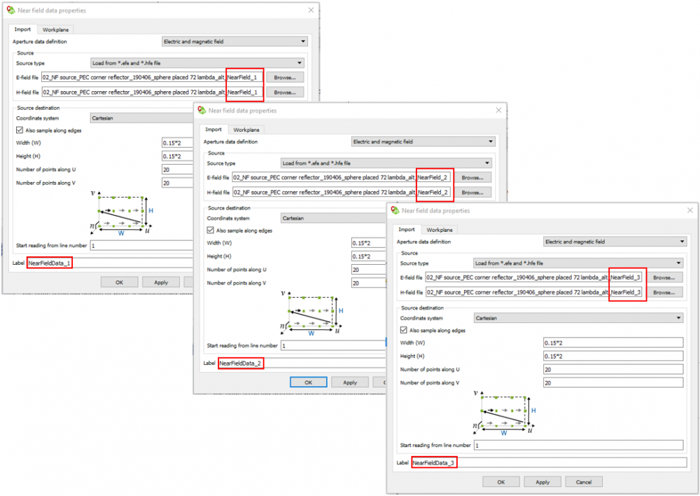
If I have three E-field and H-field data, and I would like to use it as my source in next simulation.
So I write a script as attached, however, it seemed like I must to input file named including .efe or .hfe these characters.
I want to let the input looked like this:
but I don't know how to modify this script, such as how to add additional .efe or .hfe these characters to the code as below:
properties.EFieldFilename = [[02_NF source_PEC corner reflector_190406_sphere placed 72 lambda_alt_NearField_]]..iproperties.HFieldFilename = [[02_NF source_PEC corner reflector_190406_sphere placed 72 lambda_alt_NearField_]]..i
If I use the script as shown as above, it will be looked like:
the code temp.lua seems to work. It successfully adds 3 NearFieldData in CADFEKO:
<?xml version="1.0" encoding="UTF-8"?>
What's still missing is the 'Start reading from line' which is 1 in all cases. You should change line 15
properties.ReadFromLine = '1' to properties.ReadFromLine = '1+(20*20)*'..(i-1)
20 is the number of field points in x and y, so this will ensure that the starting number will be like 1, 401, 801.
Hope this helps!
I've tried to use this .lua file to run the simulation, however, it still doesn't work, and the error message is shown as below, please check:
ERROR 30968 in line 40 of the file test2.pre: Error in opening the file 02_NF source_PEC corner reflector_190406_sphere placed 72 lambda_alt_NearField_1
To my understanding, the input characters should be like this:
02_NF source_PEC corner reflector_190406_sphere placed 72 lambda_alt_NearField_1.efe
not like this:
02_NF source_PEC corner reflector_190406_sphere placed 72 lambda_alt_NearField_1
So I would like to check with you, how can I write a propreiate code to generate the character string shown as above, such as:
02_NF source_PEC corner reflector_190406_sphere placed 72 lambda_alt_NearField_2.efe
02_NF source_PEC corner reflector_190406_sphere placed 72 lambda_alt_NearField_3.efe
I don't think that the extension (efe / hfe) are needed. However, you can do it like this:
properties.EFieldFilename = '02_NF source_PEC corner reflector_190406_sphere placed 72 lambda_alt_NearField_'..i..'.efe' properties.HFieldFilename = '02_NF source_PEC corner reflector_190406_sphere placed 72 lambda_alt_NearField_'..i..'.hfe'
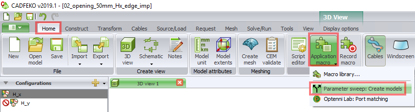
Now I have a question that, is it possible to change the size of corner reflector (s=3*c0/(fmin+f_inc*i), i=0 to 2) for each simualtion (per frequency, such as 9GHz, 10GHz and 11GHz in this case), if it can, can you help me modify this .lua file?
No, in FEKO you will always have one mesh (= one geometry) per model. You can of course use the Parameter Sweep to automatically create different models.
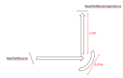
Recently, I tried to simulate a near field source radiate a signal to CATR reflector and use near field receiving antenna to receive the power of scattered field.
The schematic diagram is shown as attached, please check it.
And I found that the size of the reflector is 0.37m*0.37m, around 12 times lambda (operating frequency = 10 GHz)...if I would like to use GO method for it, it is smaller than 20 times lambda you suggest.
Due to I spent almost 2 days to solve this kind of problem by using MoM/MLFMM method, is it possible to use GO method in this case?
What is the tolerance range for this problem if I use GO method not MoM method?
Or is there any other suggestion, such as modify the setting, to boost the simulation?
20 lambda is just a rough estimation for RL-GO, it always depends on the model.
Your model seems ideal for PO or LE-PO (only one interaction on the reflector). The solution should be quite accurate. RL-GO would work but it will require much more time because the near field source will be transformed into a spherical modes source first (and same for the Rx antenna).
Just apply PO (full ray tracing) to the reflector face and you should be good. Also compare with LE-PO (full ray tracing).