1. Introduction
The shear cell is the gold standard bulk solid flowability characterisation test for quasi-static flow regime applications where the consolidating pressures are high and/or the strain rates in the bulk solid are low [1]. Examples include silo and hopper discharge as well as compaction systems like tablet presses.
Shear Cell model files can be downloaded from here:
Download Shear Cell Model .zip
Additional EDEM Calibration Kits (cone penetrometer, Dynamic and Static Angle of Repose, FT4 Rheometer, Inclined Plane Test, Rotational Shear Cell and Uniaxial compression test files can be found in this post:
EDEM Calibration Kits
Shear cell measurements are commonly used as benchmarks for the calibration of Discrete Element Method (DEM) material models for quasi-static applications[2].
Shear cell testing consists of directly shearing a bulk solid sample under confinement via a rotational or translational motion of a shear lid while applying normal stress to the lid [3], [4].
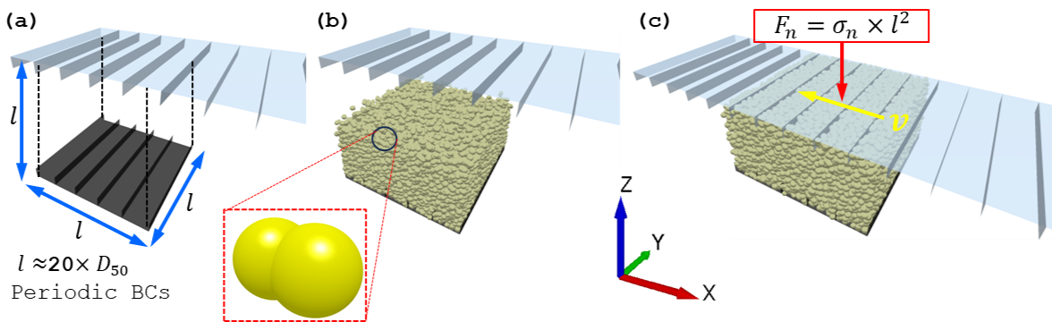
A computationally efficient approach to modeling the shear cell test using DEM is to reduce it to a periodic cell with a length scale of no less than 20 average particle diameters, as shown in Figure 1[5].
|
|---|
Figure 1: Simulation setup for shear cell test in EDEM (a) unit cell representative of bulk solid, (b) filled non-spherical particles with a normal size distribution, and (c) schematic representation of lid kinematics |
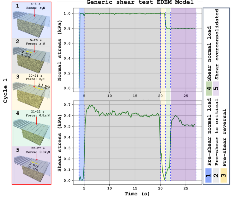
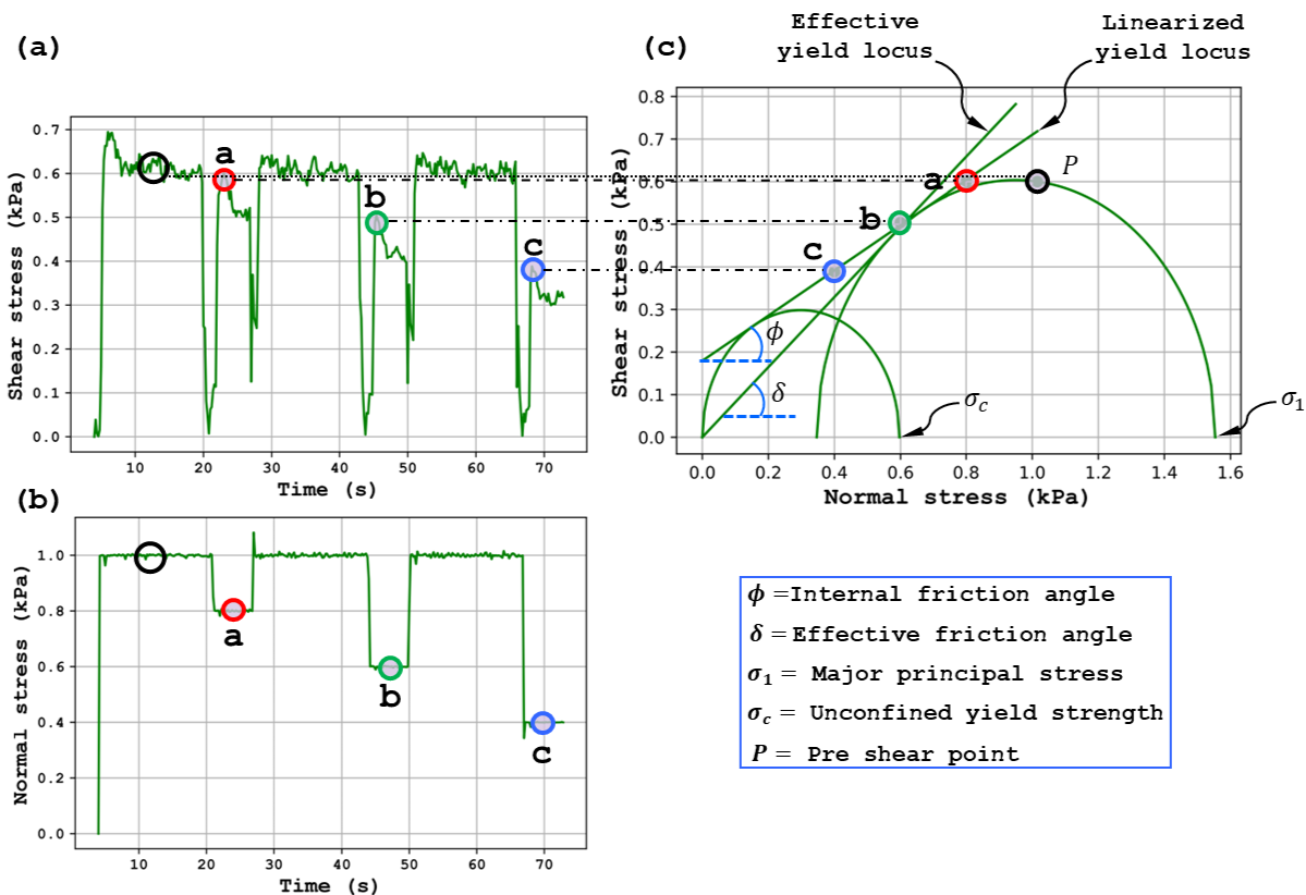
The shear cell test consists of multiple cycles, each comprising of a pre-shear stage where the material is sheared to a steady state (corresponding to the critical state) and a shear stage where the material is sheared under a reduced load (in the over-consolidated state) as shown in Figure 2. The pre-shear normal stress remains constant between cycles, but the shear normal stress is progressively reduced. Each cycle yields a point on the shear vs normal stress (σ-τ) plot. The linear fit through those points is termed the yield locus and is the fundamental measurement of the shear cell. An example of a set of yield points and the corresponding yield locus is shown in Figure 3(c) marked a, b, and c.
|
|---|
Figure 2: Exaggerated view (time step 0-27 s of 73 s simulation) highlighting various stages of cycle 1 in the shear cell simulation. |
|
Figure 3: Response of the simulation for one shear cell test highlighting the application of (a) shear stress, (b) normal stress, and (c) derived σ-τ plots representing key flow properties |
A yield locus is the yield limit of a bulk solid in the σ-τ dispace and is uniquely defined by four fundamental parameters - the major principal stress, the unconfined yield strength, the effective angle of internal friction, and the angle of internal friction. These parameters are shown in Figure 3 and can be obtained via Mohr circle analysis as follows:
- A Mohr stress circle for the normal pre-shear stress σnp, given the following, can be uniquely defined, and plotted on a σ-τ plot, as illustrated in Figure 3(c).
- The pre-shear point (P) is a point on the circumference of the Mohr stress circle.
- The Mohr stress circle is tangent and coincident with the yield locus at σ ≤ σnp.
- The center of the Mohr circle lies on the σ-axis.
- A Mohr stress circle for the unconfined yield strength σc, given the following, can be uniquely defined, and plotted on a σ-τ plot, as illustrated in Figure 3(c).
- The origin point (σ = 0 and τ = 0) is a point on the circumference of the Mohr stress circle.
- The Mohr stress circle is tangent and coincident with the yield locus.
- The center of the Mohr circle lies on the σ-axis.
- The effective yield locus is a straight line through the origin and tangent to the larger Mohr stress circle at σ ≤ σnp
The ratio of major consolidating stress σ1 to unconfined yield strength σc, termed the flow function coefficient, is a common metric for the flowability characterization of bulk solids in the quasi-static flow regime.
2. Modelling methodology
The modeling methodology for the shear cell test follows a unit cell approach similar to the one proposed by Ketterhagen et al. [5]. A representative cubic sample of the bulk solid is generated to a pre-defined solid fraction using EDEM’s volume packing tool. The sample length scale should be at least twenty times the average particle diameters to avoid artificial jamming effects. The sample is bound by two ribbed plates, as shown in Figure 1(a), where the top plate (named ‘Lid’ in the model) is movable while the bottom plate (named ‘Base’ in the model) is fixed. The 'Lid' is given translational degrees of freedom along the vertical Z and horizontal X global Cartesian directions to apply normal and shear loads to the bulk solid. Linear periodic boundaries are imposed in the X and Y global Cartesian directions to approximate plane strain conditions and enable the large shear deformations required for achieving the critical state.
The bulk solid is modeled using the two-sphere particle shape with an aspect ratio of 1.5 shown in Figure 1(b) in order to capture shear dilation in the bulk solid [6]. A normal particle size distribution with a 15 percent coefficient of variance is used to avoid artificial crystallization in the granular assembly[5]. The Edinburgh Elasto-Plastic Adhesive (EEPA) model is used to describe the particle contact mechanics. This model can capture the stress-history-dependent behavior that is characteristic of fine particulate solids and commonly quantified by the shear cell yield locus [7].
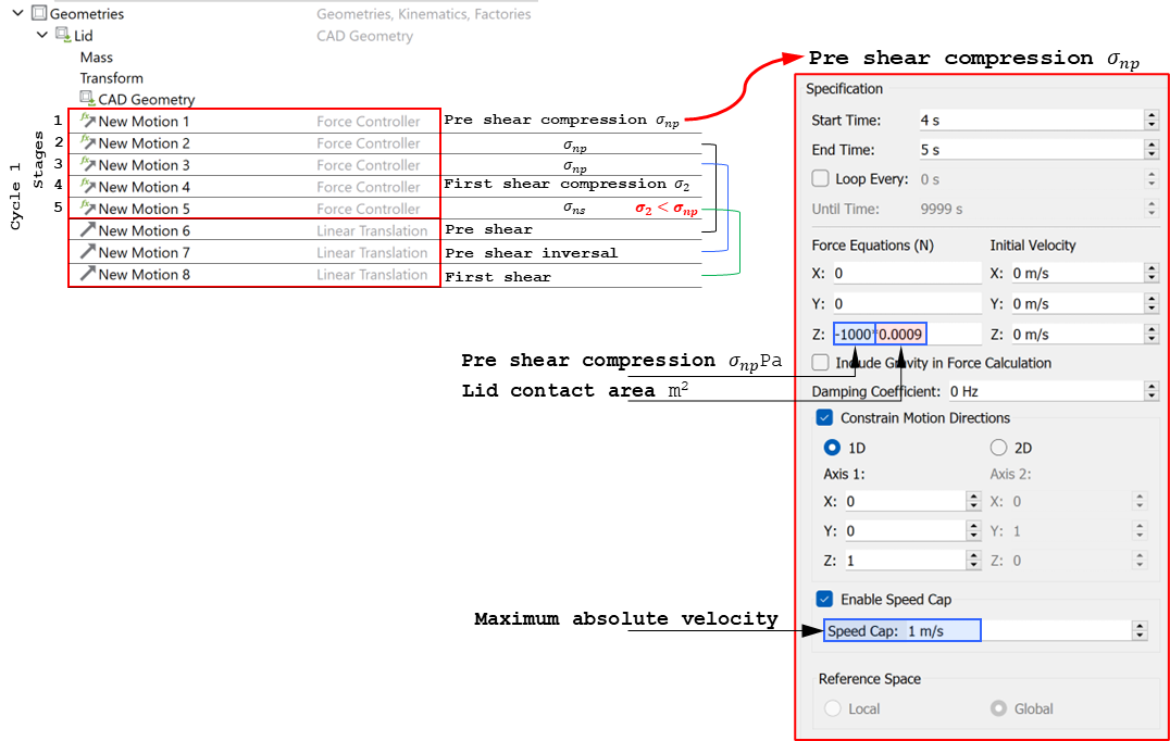
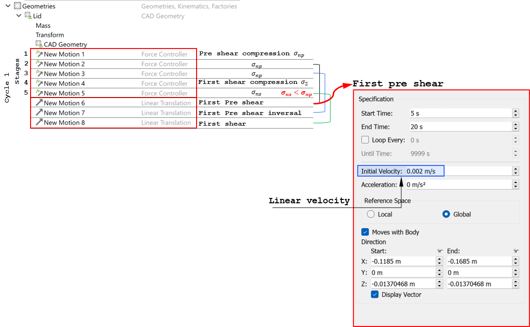
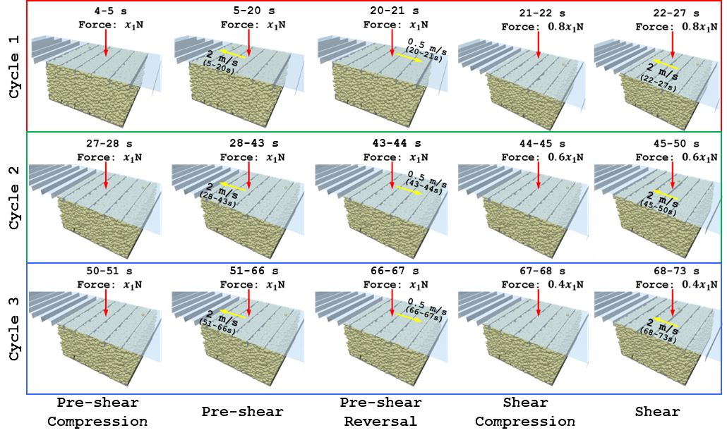
The loading sequence, described in Figure 3, is imposed on the numerical sample using EDEM’s motion controller feature. The motion controller settings corresponding to the pre-shear stage are shown in Figures 4 and 5. To achieve a controlled normal stress application a speed cap is enabled for the linear translation of the lid. This capping velocity is typically of the order of five average particle diameters per second. The sample at different stages of loading is shown in Figure 6.
|
|---|
Figure 4: Use of motion controllers to account for particle-geometry forces during normal loading of the specimen |
|
Figure 5: Use of linear translation for inducing shear in the bulk solid specimen |
|
Figure 6: Process flow for shear cell test in EDEM where x1 is the force corresponding to pre shear compression stress |
The shear cell measurements are performed in a quasi-static flow regime (strain-rate independent) and the shear rate or particle density in the simulation can be increased in the interest of computational efficiency provided that the quasi-static conditions are maintained. In practice this can be achieved by keeping the Inertial number I defined in Equation 1 within the range I<1e-3 where the inertial effects are negligible and a strain rate independent behavior consistent with the quasi-static flow regime is observed [8].

| (1) |
|---|

| (2) |
Where is the shear strain rate, d is the particle diameter, P is the hydrostatic pressure, and ρ is the bulk density. The distance between the lid and the base is l, moving at a relative velocity of v, as shown in Figure 1.
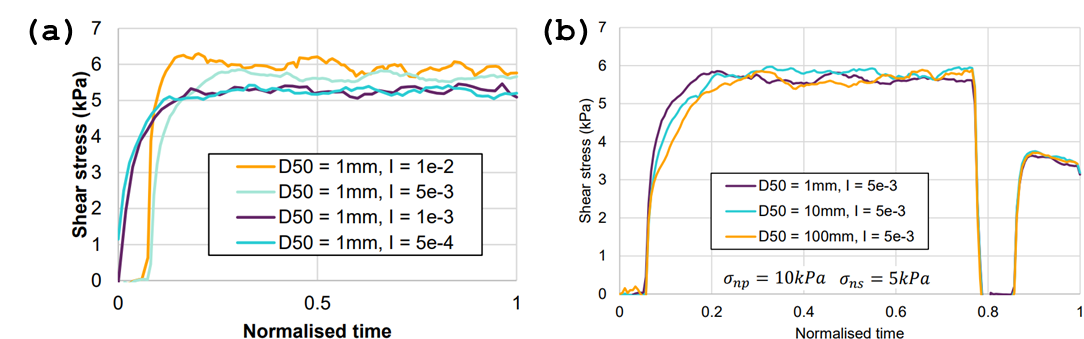
Example results for the pre-shear and shear stages of shear cell tests at varying inertial numbers are shown in Figure 7(a). It can be observed that the results are approximately constant for I < 01e-3 but the simulation time reduces linearly with I.
It is also possible to maintain the results at varying geometric scales when using the EEPA model by scaling the pull-off force and surface energy according to Equations 3 and 4 [9]. Note that the ratio of particle diameter to sample length needs to be maintained. Example results for the pre-shear and shear stages of a shear cell test at varying geometric scales are shown in Figure 7(b) and an excellent agreement can be observed over a wide range of particle diameters.
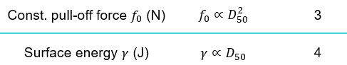
Where D is the particle diameter, f0 is the EEPA constant pull-off force, γ is the EEPA surface energy, and l is the sample length scale.
|
|---|
Figure 7: Variation of shear stress profile with varying (a) inertial number and (b) particle diameter |
3. Post-processing with EDEMpy
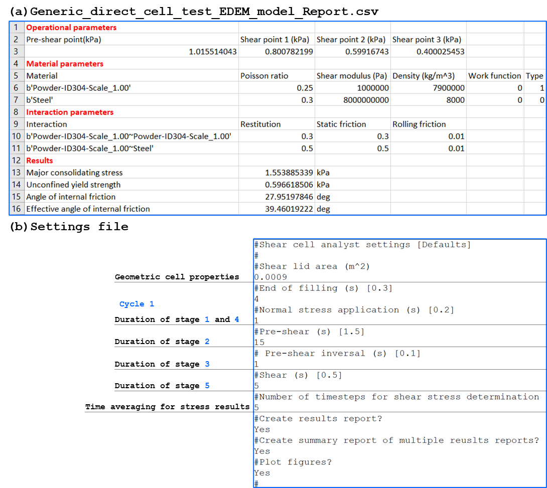
The shear test results shown in Figure 3 can be automatically exported from the completed EDEM simulations using the ‘Generic_shear_cell_test_analyst.py’ script provided with the example shear cell model here. This Python script utilizes the EDEMpy library for post-processing EDEM simulation data to compute and export the results in graphs such as the ones shown in Figure 3 and comma-delimited files like the one shown in Figure 8a.
This Python script file is accompanied by the settings file ‘Generic_shear_cell_settings.txt’ shown in Figure 8(b) which defines the key time steps for post-processing of the different test cycles as well as the required outputs.
|
|---|
Figure 8: (a) Extracted responses from the EDEM simulation deck (b) settings file read by the Python post-processing script |
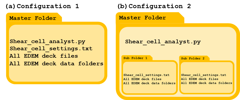
Multiple simulation decks can be post-processed by arranging files into one of two configurations, as shown in Figure 9. In configuration two (Figure 9(b)), each simulation deck can be post-processed with its custom setting file whereas, in configuration one (Figure 9(a)), a single setting file is read for post-processing of all the EDEM decks. The following sequence outlines the workflow for post-processing.
- Arrange the files as shown in Figure 9.
- Open an existing/blank EDEM simulation file and go to EDEM Analyst-->Run EDEMpy Script.
- Select ‘Generic_shear_cell_test_analyst.py’-->Run Script.
- Reports and graphs will be generated in the master folder.
|
|---|
Figure 9: Configuration of folders for post-processing using the ‘Generic_shear_cell_test_analyst.py’ script (a) single setting applicable to all EDEM decks, and (b) provision for custom settings for each simulation deck. |
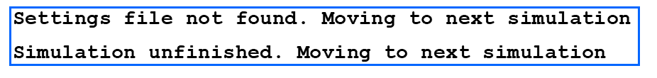
Only complete simulations with setting files will be post-processed, otherwise an error message, as shown in Figure 10, will be generated. To avoid file overwriting, all simulation files should have unique folders and simulation names.
|
|---|
Figure 10: Possible error messages that could be encountered during post-processing |
4. References
[1] D. Schulze, Powders and bulk solids, Schulze: P. Springer-Verlag Berlin Heidelberg, 2008.
[3] ASTM D6773. "Standard shear test method for bulk solids using the Schulze ring shear tester." ASTM International, p. 27, 2002. doi: 10.1520/D6773-16.
[4] ASTM Standard D6128-16 "Standard Test Method for Shear Testing of Bulk Solids Using the Jenike Shear Tester."ASTM International, p. 20. doi: 10.1520/D6128-16.
[5] W. Ketterhagen and C. Wassgren, “A perspective on calibration and application of DEM models for simulation of industrial bulk powder processes,” Powder Technol., vol. 402, p. 117301, 2022, doi: 10.1016/j.powtec.2022.117301.
[6] J. Härtl and J. Y. Ooi, “Numerical investigation of particle shape and particle friction on limiting bulk friction in direct shear tests and comparison with experiments,” Powder Technol., vol. 212, no. 1, pp. 231–239, 2011, doi:10.1016/j.powtec.2011.05.022.
[7] S. C. Thakur, J. Y. Ooi, and H. Ahmadian, “Scaling of discrete element model parameters for cohesionless and cohesive solid,” Powder Technol., vol. 293, pp. 130–137, 2016, doi: 10.1016/j.powtec.2015.05.051.
[8] G. D. R. Midi, “On dense granular flows,” Eur. Phys. J. E, vol. 14, no. 4, pp. 341–365, 2004, doi: 10.1140/epje/i2003-10153-0.
[9] S. C. Thakur, J. Y. Ooi, and H. Ahmadian, “Scaling of discrete element model parameters for cohesionless and cohesive solid,” Powder Technol., vol. 293, pp. 130–137, 2016, doi: 10.1016/j.powtec.2015.05.051.