Signal conversion

 

Signal conversion is needed to set up different types of analysis in Optistruct. FRA needs signal conversion from time to frequency domain. Another example is Random response analysis that requires definition of PSD as input function.

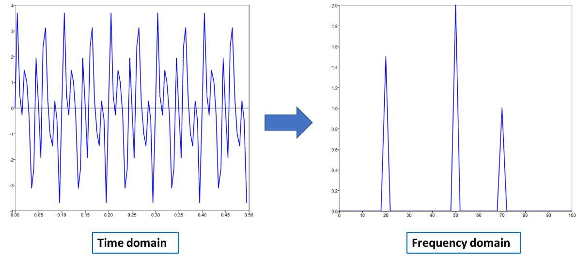
Figure 1: Signal conversion from time to frequency domain

Data manipulation can be easily done with Altair Compose, making use of Signal Viewer tool that is part of GUI utilities.

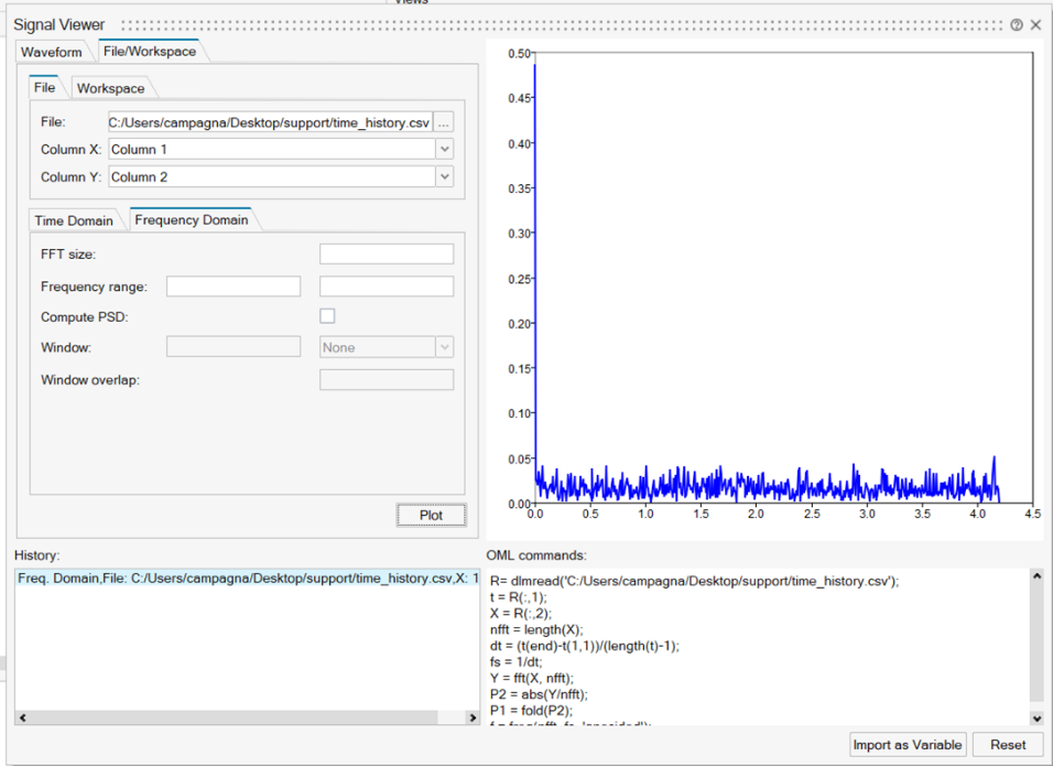
Figure 2: Signal Viewer

This tool has the capability to generate different types of Waveforms or read data from input files and covert data from time domain to frequency domain. User can specify a size for the FFT or use the dimension of the input vector and if a lowpass/highpass filter is needed an upper or lower frequency value can be defined.

For PSD computation it is possible to apply a windowing method to the signal for reducing spectral leakage.

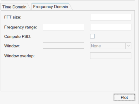
Figure 3: conversion option

 After completing the operation .oml command lines to implement the conversion are generated and can be used to create a script for future usage.

Csv and .txt format are supported for data i/o operations.

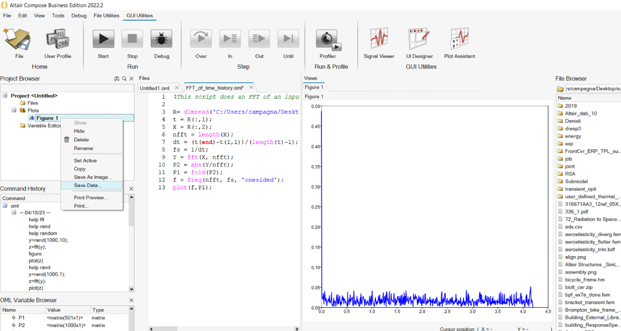
Figure 4: Data export

 

After the conversion data can be saved directly from Figures.

 

Data can be used for FE analysis with this procedure:

1. Open the FE model in HyperWorks, enable Utility Tab from View drop down menu.

 

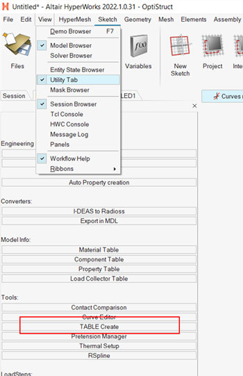
Figure 5: Utility Tab

 

2. Open Utility Tab and select Table Create.

 

3. Select Import Table and TABLED1 type for FRA or TABRND1 for Random analysis.

 

      

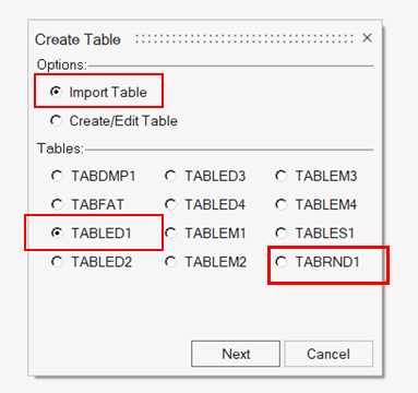
Figure 6: Create Table

 

4. Select the .csv file saved from Compose, give a name to the table and Apply.

 

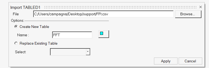
Figure 7: Import Table

 

5. A new Curves collector is created in Hyperworks db. You can review it with the Curve Editor.

 

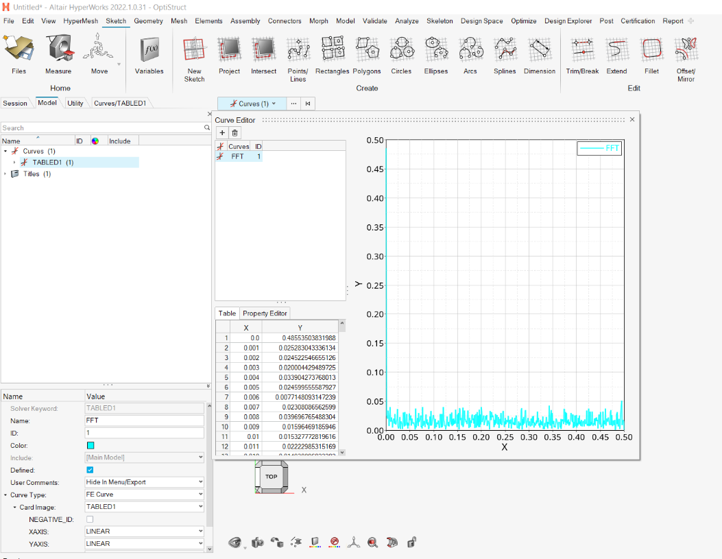
Figure 8: Curve Editor

 

6. Link the TABLED1 to an RLOAD1/2 collector with the dynamic excitation you need to apply, or the TABRND1 to a RANDPS card.

 

This will provide the load for the analysis you need to set up.