Altair PSIM is a simulation and design software for power electronics, motor drives, and power conversion systems. Altair Compose is an environment for doing math calculations, handling data, automating workflows and much more.
A new, powerful, library has been released in Compose from v2022.3 onwards, the PSIM Integration library. This library allows to seamlessly build workflows integrating both tools for running simulations in batch mode, extracting, handling, and writing results for further usage and, in general, for saving time and effort in design and simulation tasks on PSIM.
Check out the Compose - PSIM Integration starter’s guide if you haven’t already, as we go over the very basics there. In this post, we explore some other very powerful features from the PSIM Integration library, concretely, you will learn how to split simulations into multiple chunks and change the simulation time step, print time, etc. on the go to create more efficient workflows.
PSIM Schematic
The PSIM Schematic file (.psimsch) that we will be using is a simple buck converter: A DC – DC converter that is very common in power electronics. It lowers voltage applied to a load with respect to its input, while increasing current.

The results produced as outputs of this simulation are I(Q2): Current flowing through the MOSFET and Vout: Voltage at the voltage probe. All circuit components have fixed values this time.
Leveraging save & load flags
PSIM features the SAVE and LOAD functions, in which circuit voltages, currents and other quantities can be saved at the end of a simulation session and loaded back as the initial conditions for the next simulation session. This provides the flexibility of running a long simulation in several shorter stages with different time steps and parameters. Components values and parameters of the circuit can be changed from one simulation session to the other.
When running simulations from Compose, you can set these flags in the parameters definition used by the schematic.
Setting total simulation time and solver time step
Same as with save and load flags, the total simulation time and the solver time step can be declared in the parameters definition. The time step must be at least ten times faster than the fastest switching speed in the circuit. Excessively small time steps can result in long simulation times.
Setting print time and print step
Setting the print time and print step are useful for reducing the size of files produced as outputs. The print time is the point from which results will be stored in the output file, no results will be stored prior to this time. A print step of n means that only one in every n data points will be saved to the output file.
Let’s have a look at how to set these parameters in a PSIM script. First of all, let’s define the schematic to simulate and the name of the output SMV file to create.
close all, clear, clc
% Define input & output files for PSIM
input_var.FilePath = '.\buck.psimsch';
input_var.GraphFilePath = '.\buck_results.smv';
Now let’s define a parameters string for the simulation. It will contain desired simulation time, the timestep, and we will set the value of SAVEFLAG to 1. As the highest switching frequency is known to be 200 kHz, let’s define the timestep in such a way that there are 10 steps for every switching cycle, that is, the largest allowed timestep.
% Total time for simulating system's transient response
totalTime = 0.001;
% Get maximum step size that gives 10 points per cycle
Fsw = 200e3;
timeStep = (1/Fsw)/10;
% Create parameters string for simulation
input_var.Parameters = sprintf('TOTALTIME = %g\nTIMESTEP = %g\nSAVEFLAG = 1', totalTime, timeStep);
% Run PSIM simulation
simResults = PsimSimulate(input_var);
An SSF file containing the initial conditions for any subsequent simulations should have been created so, after reading all variables from the results, let’s just make sure an SSF file is indeed present in the working directory. I’m doing this just for debugging.
% Extract transient results
tTransient = simResults.Graph.Values{1};
IQTransient = simResults.Graph.Values{2};
VoutTransient = simResults.Graph.Values{3};
% Check SSF file was created
if isfile('.\buck.ssf')
disp('SSF file created succesfully');
else
error('SSF file not created');
end
Let’s now simulate further, from 1 ms to 3 ms, using the initial conditions produced by the previous simulation (using LOADFLAG). Let’s also set the timestep to half of its previous value for a more detailed response now.
% Simulate steady state with new timestep and loading SSF file
totalTime = 0.003;
timeStep = (1/Fsw)/20;
input_var.Parameters = sprintf('TOTALTIME = %g\nTIMESTEP = %g\nLOADFLAG = 1', totalTime, timeStep);
simResults = PsimSimulate(input_var);
% Extract steady-state results
tSS = simResults.Graph.Values{1};
IQSS = simResults.Graph.Values{2};
VoutSS = simResults.Graph.Values{3};
% Plot output voltage
figure(1);
plot(tTransient, VoutTransient);
hold on
plot(tSS, VoutSS);
xlabel('Time [ms]');
ylabel('Output Voltage');
legend('Transient', 'Steady-state');
% Plot switching current zoomed in
figure(2);
plot(tTransient, IQTransient, 'o-');
hold on
plot(tSS, IQSS, 'o-');
xlim([tTransient(end-20) tSS(40)]);
xlabel('Time [ms]');
ylabel('Switching Current');
legend('Transient', 'Steady-state');
Plotting both simulations’ results will illustrate the effect of these setting perfectly:
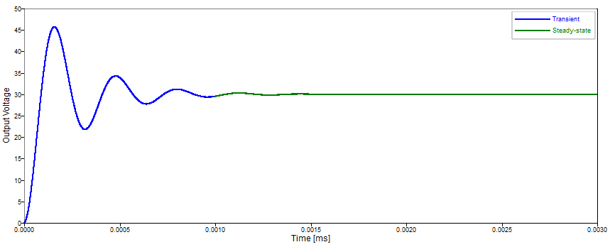

As you can see, the second simulation starts only after the time in which the first one finished and, zooming into the switching current plot, the new, smaller, time step is noticeable.
This is extremely useful. It can be used for reducing the computational burden of our simulations on segments we are not interested in or maybe we may want to initialize a system and then test many different events that occur once it’s already in steady state.
Let’s continue and repeat the full simulation now in a single chunk, but let’s set a print time such that the transient part of the simulation is not stored in the output.
% Simulate transient + steady-state at once, omit report results only from desired print time until end
timeStep = (1/Fsw)/50;
printTime = 0.002;
input_var.Parameters = sprintf('TOTALTIME = %g\nTIMESTEP = %g\nPRINTTIME = %g', totalTime, timeStep, printTime);
simResults = PsimSimulate(input_var);
% Extract steady-state results
t = simResults.Graph.Values{1};
IQ = simResults.Graph.Values{2};
Vout = simResults.Graph.Values{3};
% Plot output voltage
figure(3);
curve = plot(t, Vout, 'o-');
set(curve, 'displayname', 'Print step = 1');
hold on
Lastly, we can repeat the simulation, now setting a print step of 10 and overlay the output voltage plot for both simulations. Zooming in, this clearly shows the trade-off between output file size and fidelity that this parameter has.
% Change print step to only report every n time steps
printStep = 10;
input_var.Parameters = sprintf('TOTALTIME = %g\nTIMESTEP = %g\nPRINTTIME = %g\nPRINTSTEP = %d', totalTime, timeStep, printTime, printStep);
simResults = PsimSimulate(input_var);
% Extract steady-state results
t = simResults.Graph.Values{1};
IQ = simResults.Graph.Values{2};
Vout = simResults.Graph.Values{3};
% Plot output voltage
curve = plot(t, Vout, 'o-');
xlim([t(1), t(15)])
xlabel('Time [ms]');
ylabel('Output Voltage');
set(curve, 'displayname', sprintf('Print step = %d', printStep));
legend on

As you can see, only one in ten data points was stored in the second simulation. All these tricks are ready to be implemented in Compose and will prove very useful to take your workflows to the next level. Go ahead and leverage them under real circumstances to fully reap the benefits.
Check out the previous Compose - PSIM integration posts: